Computer Mathematics Systems and Tasks with Parameters
Yurii V. Horoshko
1 a
, Tetiana V. Pidhorna
2 b
, Petro F. Samusenko
3 c
and Hanna Y. Tsybko
1 d
1
T. H. Shevchenko National University “Chernihiv Colehium”, 53 Hetman Polubotka Str., Chernihiv, 14013, Ukraine
2
State University of Trade and Economics, 19 Kyoto Str., Kyiv, 02156, Ukraine
3
National Technical University of Ukraine “Igor Sikorsky Kyiv Polytechnic Institute”,
37 Peremohy Ave., Kyiv, 03056, Ukraine
Keywords:
Computer Mathematics Systems, Tasks with Parameters, GeoGebra, GRAN.
Abstract:
Methodological aspects of using software GeoGebra and GRAN1 for solving tasks with parameters are con-
sidered in the paper. Criteria of software selection are developed and a comparative analysis of the specified
software for solving tasks with parameters is given.
1 INTRODUCTION
Modeling of various processes and phenomena is one
of the main general methods used in scientific re-
search.
Learning to solve tasks with parameters consid-
ered in the process of teaching mathematics is one
of the preparatory stages for mathematical modeling,
where models are studied under different conditions,
in particular, under different values of the parameters
of mathematical models.
For decades, solving tasks with parameters was
usually included in the program of entry exams to
higher education institutions of Ukraine, currently
this skill is required for a successful completion of
an external independent evaluation in mathematics,
which has been held in Ukraine for more than 10
years. As evidenced by the practice and results of
pedagogical research, solving tasks with parameters
causes many difficulties for students (Ilany and Has-
sidov, 2014), more than 85% entrants at the external
independent evaluation in mathematics do not even
attempt to solve such tasks (Botuzova, 2019).
A number of publications are devoted to the
teaching method of solving tasks with parameters
(Amelkin and Rabtsevich, 2004; Gornshteyn et al.,
1992; Prus and Shvets, 2016; Gonda, 2018; Zakirova
et al., 2019).
a
https://orcid.org/0000-0001-9290-7563
b
https://orcid.org/0000-0002-1414-3489
c
https://orcid.org/0000-0002-4241-6173
d
https://orcid.org/0000-0002-1861-3003
With the development of computer technology
and corresponding software, the range of such
problems, means and methods of learning how to
solve them have expanded. Among the most fa-
mous free educational software, that provide ratio-
nal solving of tasks with parameters, GeoGebra,
Wolfram|Alpha, SageMath and GRAN can be dis-
tinguished (Bhagat and Chang, 2015; Krawczyk-
Sta
´
ndo et al., 2013; Gun
ˇ
caga, 2011; Kramarenko
et al., 2019; Kashitsyina, 2020; Hrybiuk, 2017; Kra-
marenko, 2005; Pokryshen, 2007; Ivashchenko, 2015;
Zhaldak, 2016).
The topic of research publications on the use of
software for the analysis of mentioned tasks covers
various aspects of teaching methods for solving tasks
with parameters: studying the forms of graphs of
functions for different values of the parameter (Ilhan,
2013; Boži
´
c et al., 2021); using a computer to illus-
trate analytical solutions (Pokryshen, 2007; Gun
ˇ
caga,
2011); the method of organizing the research activ-
ity of pupils and students in the process of prelimi-
nary graphic analysis of tasks solutions with the fur-
ther analytical solution (Kramarenko, 2005; Hrybiuk,
2017; Kramarenko et al., 2019; Krawczyk-Sta
´
ndo
et al., 2013; Gornshteyn et al., 1992); obtaining solu-
tions of the tasks based on detailed graphical analysis
(Ivashchenko, 2015; Zhaldak, 2016). As a rule, the
cited works consider examples of tasks, where solu-
tions can be obtained analytically, but this is an ex-
ceptional case in practice.
Despite the fact that a large number of studies
on mathematics teaching methods have been devoted
to this topic, in particular with the use of modern
768
Horoshko, Y., Pidhorna, T., Samusenko, P. and Tsybko, H.
Computer Mathematics Systems and Tasks with Parameters.
DOI: 10.5220/0012067700003431
In Proceedings of the 2nd Myroslav I. Zhaldak Symposium on Advances in Educational Technology (AET 2021), pages 768-780
ISBN: 978-989-758-662-0
Copyright
c
 2023 by SCITEPRESS – Science and Technology Publications, Lda. Under CC license (CC BY-NC-ND 4.0)

computer-oriented technologies, its importance is un-
doubtful, since the number of mentioned tasks and
their types is constantly increasing. It is clear that for
practical use it is important to know not so much the
exact solution value of the task, which describes the
mathematical model of a real process or phenomenon,
but whether the task is compatible and stable. Then,
with the use of modern software, it is possible to find
an approximate value of a certain solution of the task
with a predetermined accuracy, and that is quite suffi-
cient for practice.
In this work there have been developed criteria for
the selection of software, advisable for the use in the
process of solving tasks with parameters.
The work contains examples of solving such tasks
by both analytical and graphical methods. Consider-
able attention is paid to the tasks that cannot be solved
by analytical methods. At that, the plotting of quite
complex graphs of functions for different values of
parameters with the use of appropriate software helps
to avoid errors in the plotting of such graphs, to fo-
cus attention on the analysis of their form and to find
the answer to the task question. Examining tasks that
can be solved only approximately with the use of the
graphic method expands the students’ understanding
that in the process of describing mathematical models
of various objects and phenomena, such solutions are
used as well.
2 COMPUTER MATHEMATICS
SYSTEMS FOR SOLVING
TASKS WITH PARAMETERS
Let’s consider the conditions of selection and use
of computer mathematics systems (CMS) for solving
tasks with parameters.
Today, web-oriented software, including CMS, is
being used more and more. As already mentioned,
the software tools GeoGebra, Wolfram|Alpha, Sage-
Math, etc are among the most popular freely dis-
tributed computer mathematics systems.
Wolfram|Alpha is a knowledge base of various
scientific fields, including mathematical ones. It is
based on various algorithms and technologies of arti-
ficial intelligence. The web-based version can be ac-
cessed at https://www.wolframalpha.com/.
SageMath is a free and open source math system
licensed under the GPL. The web-based version can
be accessed via the link https://www.sagemath.org/.
One of the most widespread educational computer
mathematics systems in Ukraine is the software com-
plex GRAN, as evidenced by a significant number
of scientific and pedagogical publications devoted to
various aspects of the organization and implementa-
tion of the educational process in modern learning
conditions.
The software complex GRAN was developed at
the National Pedagogical Dragomanov University un-
der the leadership of M. I. Zhaldak. This com-
plex consists of three programs: GRAN1, GRAN2D,
GRAN3D.
The GRAN1 program is intended for graphic anal-
ysis and solving tasks related to the plotting of graphs
of functions on the Cartesian plane, defined explic-
itly and implicitly, parametrically, tabularly, in the po-
lar coordinate system; for processing statistical data,
plotting graphs of the probability distribution func-
tions of random variables, calculating definite inte-
grals, the length of curves, the area of curved trape-
zoids, the area of surfaces and volumes of bodies of
rotation, etc.
The first version of the GRAN1 was developed
for the Yamaha personal computer back in 1990 by
A. V. Penkov (Zhaldak et al., 2016). Later, GRAN1
was improved and adapted for use under the operat-
ing system of the Windows family by Y. V. Horoshko.
In 2019, this software tool was laid out on a re-
mote desktop, which allows it to be used through a
browser remotely (Zhaldak et al., 2021), and not only
on local computers. The GRAN-2D program is in-
tended for graphical analysis of systems of geomet-
ric objects on a plane, and the GRAN-3D program is
intended for graphical analysis of systems of three-
dimensional geometric objects. The first versions of
the GRAN-2D and GRAN-3D programs were devel-
oped in 2002. The complex is freely distributed and
can be downloaded from the website https://zhaldak.
fi.npu.edu.ua/.
One of the most common educational computer
mathematics systems is the GeoGebra system. The
first version of GeoGebra was developed in 2001-
2002 by M. Hohenwarter (Hohenwarter and Fuchs,
2004). In December 2021, GeoGebra was acquired by
the conglomerate Byju’s (Singh, 2021). This software
tool can be used both remotely and on a local com-
puter by downloading the appropriate program mod-
ules. A component of the GeoGebra system are pro-
grams for graphic analysis and solving tasks related
to the plotting graphs of functions on the Cartesian
plane, defined in explicit or implicit form, in the po-
lar coordinate system, tasks in the theory of probabil-
ity, planimetry and stereometry. Using CMS GeoGe-
bra, one can also create didactic materials for different
users, provide access to them for others; create an ed-
ucational classroom environment for students to use.
The table 1 analyzes the presence of program
Computer Mathematics Systems and Tasks with Parameters
769

functions, which, in our opinion, are needed for
graphical analysis of solving tasks with parameters.
Thus, it is advisable to use, first of all, GRAN1
and GeoGebra from the listed software tools for solv-
ing tasks with parameters. We will give appropriate
examples.
3 SOME EXAMPLES
1. Solve the equation
1 −
3
x + a −1
=
5a
(x + a −1)(x +1)
. (1)
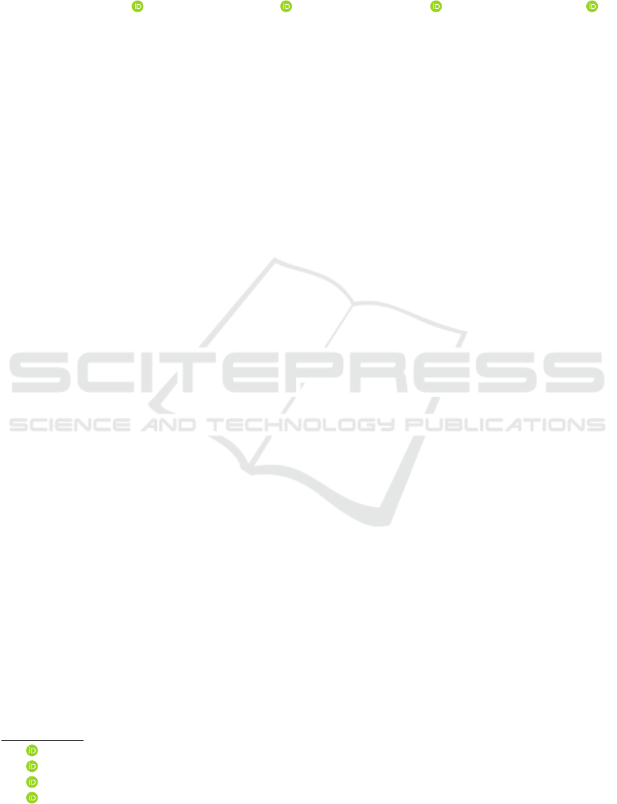
To analyze the task, we will use CMS GRAN1.
Let’s plot graphs of functions
f (x) = 1 −
3
x + a −1
and
g(x) =
5a
(x + a −1)(x + 1)
for specific values of the parameter a. To do this, we
specify the parameter a by p1 (the default parame-
ter name). Changing the values of the p1 parameter,
for example, from −5 to 5 with a step 0.1 (these val-
ues are set by default) leads to a corresponding shape
change of the graphs of the specified functions. The
equation (1) solutions are the abscissas of the points
of intersection of the graphs of the functions f (x) and
g(x). Since for values of the parameter p1 from −4.9
to −3.1, from −2.9 to −0.1 and from 0.1 to 5 the
graphs of the functions f (x) and g(x) intersect at two
points, the equation (1) for such p1 has two solutions
(figure 1).
If p1 = −5, then visually the graphs of the func-
tions intersect at one point, that is an exceptional case
for the equation (1), since it, generally speaking, re-
duces to a quadratic equation, and therefore, under
certain conditions, has two solutions. Therefore, it is
advisable to consider the p1 parameter, for example,
from −6 to 5.
Considering the shape of the graphs of the func-
tions f (x) and g(x) for p1 = −5.2, p1 = −5.1, p1 =
−4.9 and p1 = −4.8 and taking into account, that
even increasing the scale for p1 = −5 it is not pos-
sible to get a clear answer about the number of roots
of the equation (1) (figure 2), we come to the conclu-
sion about the need of analytical equation study (1)
when the value of the parameter a is changing in a
neighborhood of the point −5.
In the case when p1 equals −3 or 0 the graphs of
the functions f (x) and g(x) intersect at one point, that
is, the equation (1) has a unique solution (figure 3,
figure 4).
Taking into account the continuity of the func-
tions f (x) and g(x) on the corresponding intervals,
it is possible to hypothesize about the existence of
two solutions of the equation (1) for a ∈ (−∞;−5) ∪
(−5;−3)∪(−3;0)∪(0;∞) and about the existence of
one solution of the equation (1) for a = −5, a = −3
and a = 0. To confirm or refute it, as a rule, it is nec-
essary to make an analytical study of the problem.
We present the analytical solution of the given
equation. It is clear that x ̸= −1, x ̸= 1 −a. Then
(x + a −4)(x + 1) −5a = 0
or x
2
+ x(a −3) −4a −4 = 0.
According to Viet’s theorem
x
1
= 4, x
2
= −a −1.
From the restrictions imposed on the variable x, it fol-
lows that
x
1
̸= −1, x
1
̸= 1 −a, x
2
̸= −1, x
2
̸= 1 −a.
The first and fourth conditions are obvious. There-
fore, let’s consider the rest of the conditions in more
detail. From the inequality x
1
̸= 1 −a we get that
a ̸= −3. That is for a = −3 the value x
1
= 4 is not
a root of the given equation (in this case, the root will
be x
2
= 2) (figure 2). The third inequality x
2
̸= −1 is
equivalent to a ̸= 0. Therefore, for a = 0 the root of
the equation will be x
1
= 4 (figure 3).
Thus, if a = −3, then x = 2 (figure 2), if a = 0,
then x = 4 (figure 3), and if a ̸= −3 and a ̸= 0, then
x = 4 or x = −a −1 (figure 1).
Thus, the previously proposed hypothesis about
the number of roots of the equation (1) was partially
confirmed.
In figures 1-3 the parameter value respectively is
0.4, −5 and −3. Note that the parameter value can
also be selected using a slider. At that, the same draw-
ing can contain images of graphs of functions that cor-
respond to different fixed values of the parameter.
As it is known, there exists a slightly different ap-
proach to constructing a geometric interpretation of
the task (1). Namely, it is necessary to find the inter-
section points of the graph of the function
h(x) = 1 −
3
x + a −1
−
5a
(x + a −1)(x + 1)
for different values of the parameter a with the ab-
scissa axis. It is clear that solving such a task using
appropriate software is similar in complexity to the
presented above. In figure 5 the graph of the function
h(x) is plotted under the condition that a = 0.4. In
this case the graph of the function h(x) intersect the
abscissa axis at two points, that is, the equation (1)
has two solutions.
AET 2021 - Myroslav I. Zhaldak Symposium on Advances in Educational Technology
770

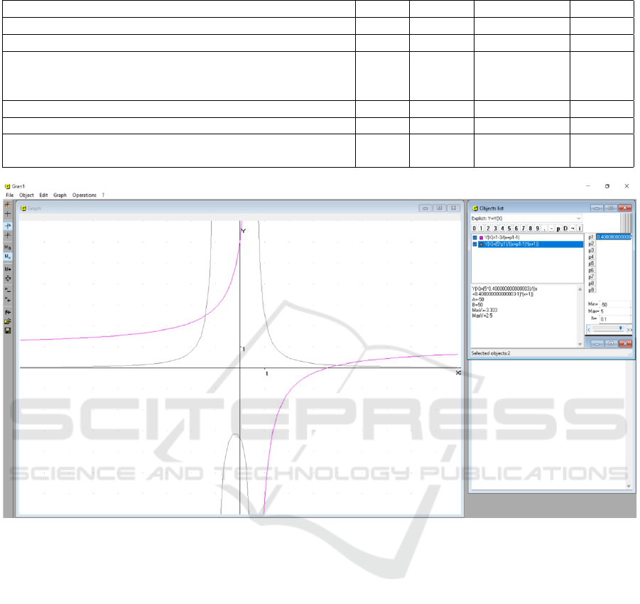
Table 1: Program comparison.
Program functions GRAN1 GeoGebra Wolfram|Alpha SageMath
Plotting graph of a function given in explicit form + + + +
Plotting graph of a function given in implicit form + + + +
Using a parameter in the function definition and its change,
automatic change of a graph depending on the parameter
value, the possibility to change the parameter changing step
+ + – –
Plotting of a tangent to a curve at a point + + + +
Ability to change the scale + + - –
Determination of the coordinates of the intersection of graphs
of functions
+ + + –
Figure 1.
Note that the use of this approach to solving tasks
with parameters can lead to a more adequate geomet-
ric interpretation of the task. So, for a = −5 the graph
of the function h(x) at the point with abscissa x = 4
touches the abscissa axis (figure 6).
This means that
h(4) = 0, h
′
(4) = 0,
i.e. the equation
h(x) = 0,
and therefore the equation (1) has two identical roots
x = 4. Indeed, by construction
h(x) = (x −4)
2
e
h(x),
e
h(4) ̸= 0.
2. Find the number of roots of the equation
a
x
= log
a
x. (2)
In this case, we use GeoGebra software for
graphic illustrations. Let’s plot the graphs of the func-
tions f (x) = a
x
and g(x) = log
a
x for specific values of
the a parameter. Increasing the value of the parameter
a from 0 with a step of 0.1, we come to conclusion –
if the parameter a takes values from 0.1 to 0.9, then
the equation (2) has one root, from 1.1 to 1.4 – the
equation (2) has two roots, and finally, if the parame-
ter value is greater than 1.4, then the equation (2) has
no roots.
It is clear that the use of only a graphical way of
solving the equation (2) does not only not allow to
make the correct conclusion about the number of roots
of the equation for a ∈ (0; 1) ∪(1; ∞), but also does
not allow us to express an adequate hypothesis about
the length of the intervals of change of the parame-
ter a, where the equation (2) has the same number
of roots. And the situation is not improved by a sig-
nificant decrease in the step of changing the parame-
Computer Mathematics Systems and Tasks with Parameters
771

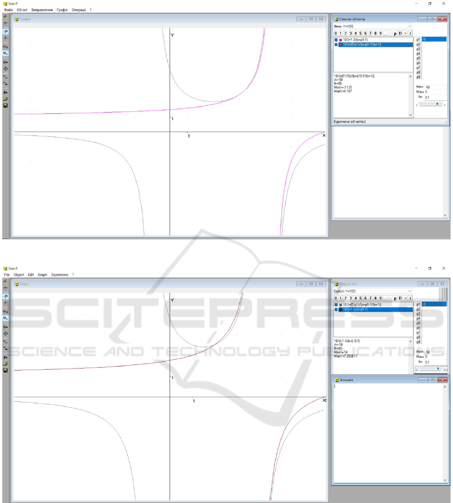
Figure 2.
Figure 3.
ter a, since the values of the parameter, when passing
through which the number of roots of the equation (2)
changes, are transcendental numbers.
Therefore, an analytical study of the task is neces-
sary.
On the condition of the task x ∈ (0;∞) and a ∈
(0;1) ∪(1;∞). Let it first a ∈ (1; ∞). We find a tan-
gent point M of graphs of the functions y = a
x
and
y = log
a
x. It is clear that the abscissa of the tangent
point will be the solution of the equation (2). Since
these functions are mutually turned, their graphs are
symmetrical relative to the line y = x. Taking into
account the strict monotony of functions y = a
x
and
y = log
a
x and the immutability of the type of con-
vexity of their graphs, we come to the conclusion that
if the tangent point of the graphs of these functions
AET 2021 - Myroslav I. Zhaldak Symposium on Advances in Educational Technology
772

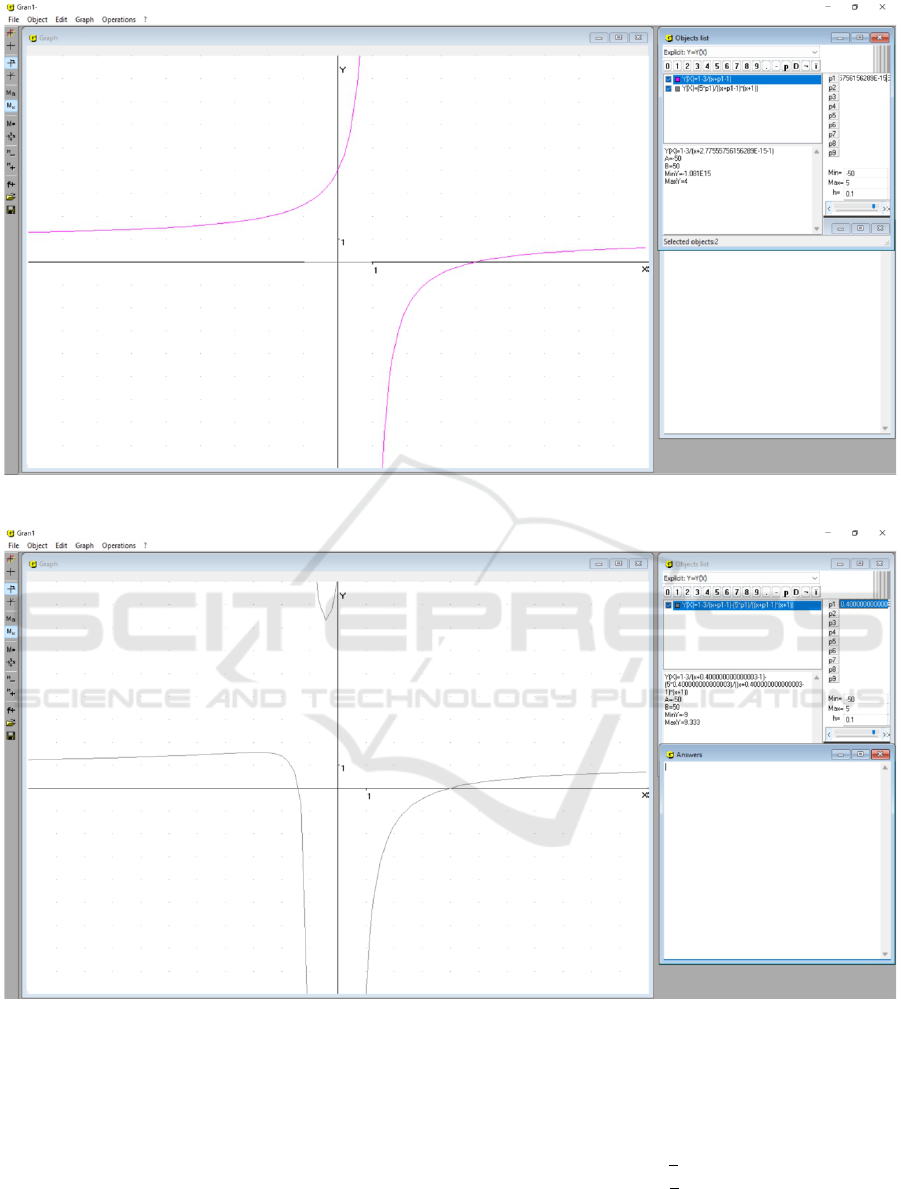
Figure 4.
Figure 5.
exists, then it is unique and lies on the line y = x (fig-
ure 6).
It is known that the coordinates of the tangent
point of graphs of the functions y = ϕ(x) and y = ψ(x)
meet the system of equations

ϕ(x) = ψ(x),
ϕ
′
(x) = ψ
′
(x),
that in our case will look like

a
x
= x,
a
x
lna = 1.
From here we get a =
e
√
e, M(e, e).
Suppose, that a >
e
√
e. Then graphs of the func-
tions y = a
x
and y = x do not intersect, that is, the
equation (2) has no solution (figure 8).
Computer Mathematics Systems and Tasks with Parameters
773

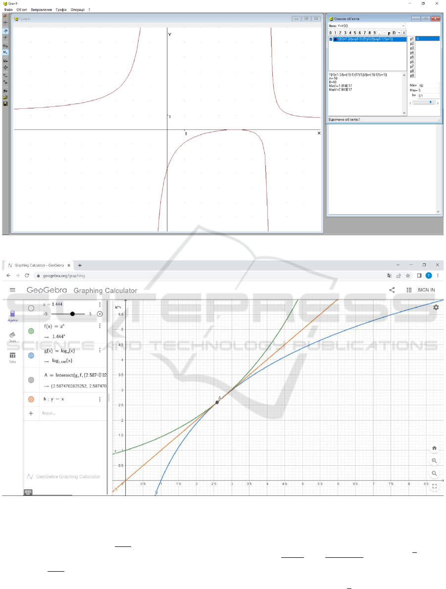
Figure 6.
Figure 7.
Indeed, we denote as h(x) = a
x
−x, x ≥ 0. Then
h
′
(x) = a
x
lna −1 and x = −
lnlna
lna
is a stationary point
of function h(x). Since h
′′
(x) = a
x
ln
2
a > 0, x ≥ 0,
then x = −
lnlna
lna
is a minimum point of the function
h(x).
Taking into account that
h(0) = 1 > 0
and
h

−
lnln a
lna

=
1 + ln ln a
lna
> 0, a >
e
√
e,
then h(x) > 0, x ≥ 0, i.e. a
x
> x, x ≥0.
Let it now be 1 < a <
e
√
e. Then the equation (2)
has two solutions.
Indeed, determining the function h(x), like before,
AET 2021 - Myroslav I. Zhaldak Symposium on Advances in Educational Technology
774

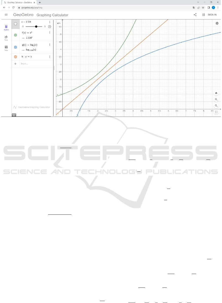
Figure 8.
we get
h(0) = 1 > 0, h

−
lnln a
lna

< 0,
lim
x→+∞
h(x) = +∞.
Since graphs of the functions y = a
x
and y = log
a
x
have no points of inflection, then according to the
Bolzano-Koshi theorem, they intersect at two points
that are besides contained on the line y = x (figure 9).
Let 0 < a < 1. We denote as l(x) = log
a
x −a
x
,
a ∈ [a
0
;1), where a
0
will be determined below. Let’s
investigate the function l(x) on monotony:
l
′
(x) =
1 −xa
x
ln
2
a
x lna
.
The value a
0
we select so that l
′
(x) ≤ 0, x ∈ (0;∞).
Since x ln a < 0, x ∈ (0;∞), a ∈ (0;1), then l
′
(x) ≤
0, x ∈ (0;∞), than and only when
1 −xa
x
ln
2
a ≥ 0, x ∈ (0; ∞).
Select a
0
so that
1 −xa
x
ln
2
a ≥ 0, x ∈ (0; ∞), a ∈[a
0
;1).
We denote as m(x) = xa
x
ln
2
a, x ∈ (0; ∞) and in-
vestigate m(x) per extremum. Calculating
m
′
(x) = a
x
ln
2
a(1 + x ln a),
m
′′
(x) = a
x
ln
3
a(2 + x ln a),
we are convinced, that the stationary point x = −
1
lna
of the function m(x) is a maximum point.
Since
m(0) = 0
and
m

−
1
lna

= −
1
e
lna ≤−
1
e
ln
1
e
e
= 1, a ∈

1
e
e
;1

,
then a
0
=
1
e
e
.
Thus, l
′
(x) ≤ 0, x ∈ (0; ∞), and points where
l
′
(x) = 0, do not form a segment. Therefore, the func-
tion l(x), x ∈(0; ∞), a ∈

1
e
e
;1

is descending. There-
fore, the equation (2) has one solution (figure 10).
Let it finally a ∈

0;
1
e
e

. In this case, the equation
(2) has three solutions (figure 11).
Indeed, graphs of the functions y = a
x
and y =
log
a
x intersect at some point of the line y = x. Let us
denote the abscissa of this point as x
0
. It is clear that
x = x
0
is a solution of the equation (2). Consider the
interval (0; x
0
). Note that lim
x→0+
l(x) = +∞. Determine
a sign of the number l(x
0
−ε), where ε – is a quite
small positive constant.
l(x
0
−ε) = log
a
(x
0
−ε) −a
x
0
−ε
= log
a

1 −
ε
x
0

+
+log
a
x
0
−a
x
0
a
−ε
= x
0
+
1
lna
ln

1 −
ε
x
0

−x
0
a
−ε
=
=
1
lna
ln

1 −
ε
x
0

−x
0

a
−ε
−1

=
=
1
lna
−
ε
x
0
−
1
2

ε
x
0

2
−
1
3

ε
x
0

3
−...
!
−
Computer Mathematics Systems and Tasks with Parameters
775

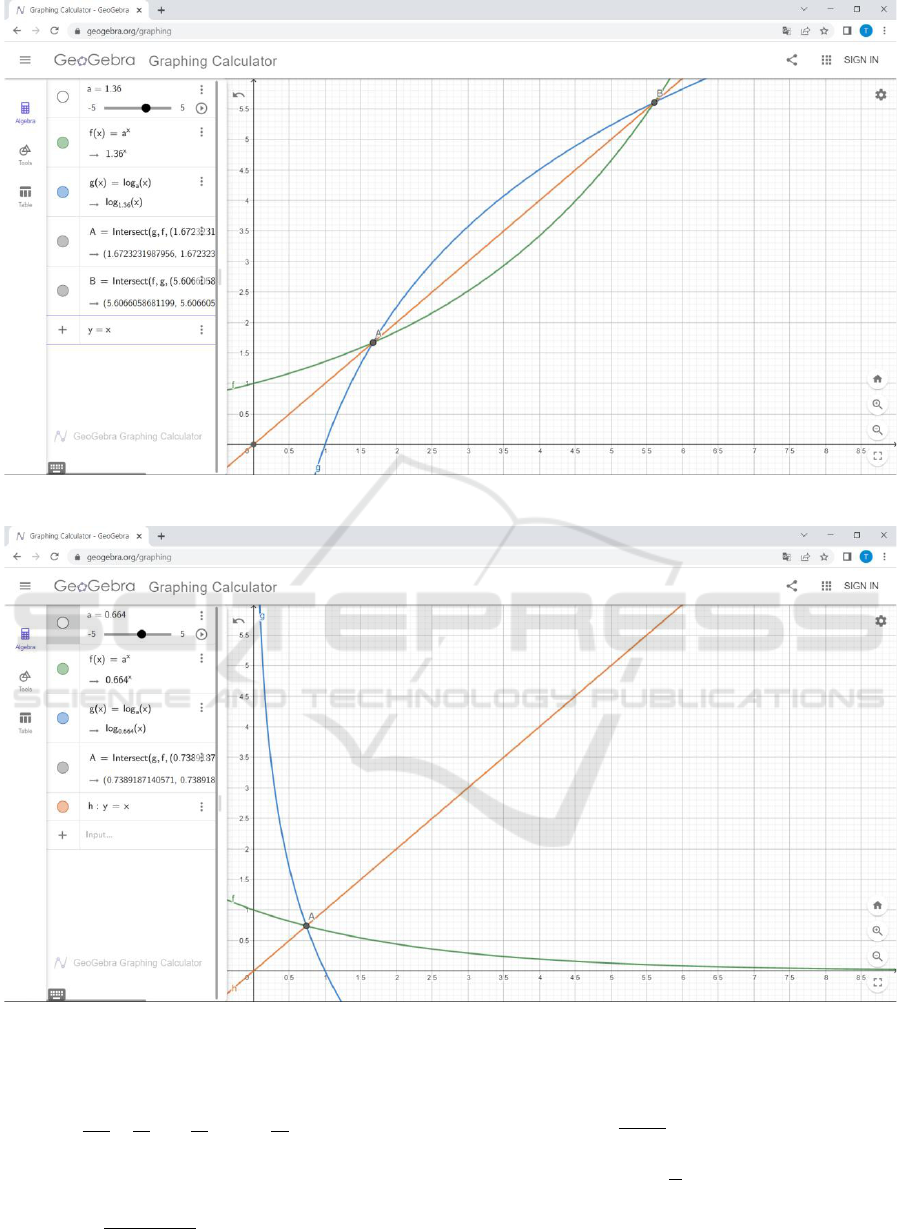
Figure 9.
Figure 10.
−x
0
(−εln a + O(ε
2
)) ≤
≤ −
1
lna
ε
x
0
+

ε
x
0

2
+

ε
x
0

3
+ ...
!
−
−x
0
(−εln a + O(ε
2
)) =
= ε

−
1
(x
0
−ε) ln a
+ x
0
lna

+ O(ε
2
) < 0,
since inequality
−
1
x
0
lna
+ x
0
lna < 0 (3)
is correct for all a ∈

0;
1
e
e

. Indeed, inequality (3) is
equivalent to
x
2
0
ln
2
a > 1
AET 2021 - Myroslav I. Zhaldak Symposium on Advances in Educational Technology
776

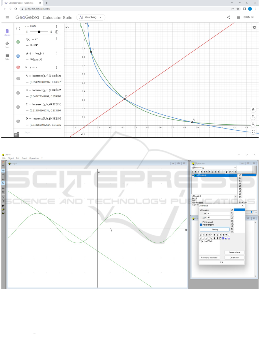
Figure 11.
Figure 12.
or to
ln
2
x
0
> 1,
i.e. x
0
∈

0;
1
e

∪(e; ∞).
Since x =
1
e
is a solution of the equation
log
1
e
e
x = x,
then the solution of the equation
log
a
x = x
is less than
1
e
, if 0 < a <
1
e
e
. And therefore x
0
∈

0;
1
e

,
that is inequality (3) is correct.
Thus, according to the Bolzano-Cosh Theorem
the equation (2) in the interval (0; x
0
) has a solution.
For reasons of symmetry, taking into account the im-
mutability of the type of convexity of graphs of the
functions y = a
x
and y = log
a
x, it follows that for
a ∈

0;
1
e
e

equation (2) has three solutions.
Computer Mathematics Systems and Tasks with Parameters
777

Summarizing the analysis we come to the conclu-
sion. Equation (2) has three solutions if a ∈

0;
1
e
e

,
two solutions if a ∈ (1;
e
√
e), one solution if a ∈

1
e
e
;1

∪
{
e
√
e
}
and has no solution if a ∈

1
e
e
;∞

.
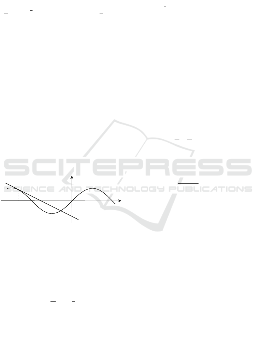
3. Find the values of the parameters a and b, for which
the equation
sinx = ax + b (4)
has two solutions.
The equation (4) will have two solutions if graphs
of the functions y = sin x and y = ax + b will inter-
sect at two points. It is clear that one of these points
is the tangent point of the graphs of these functions
(figure 12).
In the GRAN1 program, it is possible to plot a tan-
gent to a curve at a given point. In this case, the ab-
scissa of the point of tangency can be considered a pa-
rameter. Further, by gradually changing the value of
the parameter, one can observe the change in the posi-
tion of the tangent and visually determine the number
of roots of the considered equation. So, for which
values of the parameters a and b does the equation (4)
have 2 solutions?
Let the point with the abscissa x
1
is a tangent point
of graphs of the functions y = sin x and y = ax + b.
Also suppose that the solutions of the equation (4) be-
long to the segment

−
3π
2
;0

.
x
x
y
0
b
a
b
-
Figure 13.
Then the parameters a and b meet the inequalities

−1 < a < 0,
−π < b < 0.
Since

sinx
1
= ax
1
+ b,
cosx
1
= a,
then, using the basic trigonometric identity, we get
cos
r
1
a
2
−1 +
b
a
!
= a. (5)
Note that the inverse statement is correct as well.
Namely, from the condition (5) it follows that at the
point with the abscissa
x
1
= −
r
1
a
2
−1 −
b
a
graphs of the functions y = sinx and y = ax +b touch.
The line y = ax + b intersects the abscissa axis at
the point

−
b
a
;0

. Then when meeting the condition
−π < −
b
a
< 0,
the line y = ax + b and the curve y = sin x will only
have two common points.
Thus, if
(
cos

q
1
a
2
−1 +
b
a

= a,
aπ < b < 0,
then the equation (4) has two solutions.
Thinking similarly, one can find the conditions,
under which there exist two solutions of the equation
(4) at an arbitrary interval from the range (−∞;+∞)
so that at the whole range (−∞; +∞) the equation (4)
would have two solutions.
Note that the equation (4) can be solved approx-
imately with the use of expansion of the function
y = sin x in a Maclaurin series, namely,
x −
x
3
3!
+
x
5
5!
−... = ax + b. (6)
Then, taking into account the convergence of the
series in the left side of equality (5) in the range
(−∞;+∞), instead of of the equation (5) such equa-
tion can be considered
p
∑
k=1
x
2k−1
(2k −1)!
= ax + b, (7)
where the expression in the left part is a polynomial.
The value of p is determined by the specified accu-
racy.
The equation (7) contains a polynomial of an odd
degree with real coefficients. Therefore, it has an odd
number of real roots. The latter fact in no way con-
tradicts the proven statement of the even number of
real roots of equation (4), since the equation (4) un-
likely (7) is transcendental and the properties of the
function y = sinx (limited, monotony, bulge) are sig-
nificantly different from the corresponding properties
of the polynomial
p
∑
k=1
x
2k−1
(2k−1)!
.
Using the developed approach to solving the equa-
tion (4), it is possible to consider various problems
related to finding a given number of their solutions.
4 CONCLUSIONS AND FURTHER
RESEARCH PROSPECTS
The graphical method of finding solutions of equa-
tions, inequalities and their systems is based on the
AET 2021 - Myroslav I. Zhaldak Symposium on Advances in Educational Technology
778

procedure of plotting graphs of the corresponding
functions. In the case of implicit or parametric defini-
tion of functions, the process of plotting their graphs
is quite complicated. The task becomes even more
cumbersome if it contains a parameter. That is why
they often try to solve these problems using various
software tools.
This paper substantiates the expediency of using
GRAN1 and GeoGebra computer mathematics sys-
tems for solving tasks with parameter. In the GRAN1
program, it is possible to write the formula of the
function with the designation of parameters through
the variables p1, p2, . . . , p10. At that, the parameter
can be changed both by assigning it a certain value
and by using a slider. In the process of changing the
parameter values, the graph of the function is auto-
matically constructed, taking into account the updates
of the parameter values. Similar functions are inher-
ent in the GeoGebra program. It is only needed to
define the variables through which the parameters are
denoted.
Using the automatic change of the shape of the
graph for different values of the parameter, the change
of the step of changing the value of the parameter, the
change of scale for viewing the graph of the function
or its fragment, the automatic determination of the co-
ordinates of the point of intersection of the graphs of
the functions, in the work there are established the
conditions of compatibility of the geometric character
of three illustrative tasks with the parameter and their
analytical solutions are given. At that for geomet-
rical support of the process of solving the specified
tasks, GRAN1 and GeoGebra computer mathematics
systems were used, as already mentioned above. The
mentioned software tools are equally convenient for
use in the process of solving tasks with parameters.
REFERENCES
Amelkin, V. V. and Rabtsevich, V. L. (2004). Tasks with
parameters. Asar, Moscow.
Bhagat, K. K. and Chang, C.-Y. (2015). Incorporating
GeoGebra into Geometry learning-A lesson from In-
dia. EURASIA Journal of Mathematics, Science and
Technology Education, 11(1):77–86. https://doi.org/
10.12973/eurasia.2015.1307a.
Botuzova, Y. V. (2019). Parametric tasks in the con-
text of STEM-education. In Problems of mathemat-
ics education (PMO-2019): materials of the interna-
tional scientific and methodological conference, pages
237–238, Cherkasy. http://dspace.cuspu.edu.ua/jspui/
handle/123456789/3392.
Boži
´
c, R., Taka
ˇ
ci, Ð., and Stankov, G. (2021). Influence of
dynamic software environment on students’ achieve-
ment of learning functions with parameters. Inter-
active Learning Environments, 29(4):655–669. https:
//doi.org/10.1080/10494820.2019.1602842.
Gonda, D. (2018). Analysis of the causes of low achieve-
ment levels in solving problems with parameter. Eu-
ropean Journal of Education Studies, 4(4):339–354.
https://doi.org/10.5281/zenodo.1218119.
Gornshteyn, P. I., Polonskyi, V. B., and Yakir, M. S. (1992).
Tasks with parameters. Tekst, Kyiv.
Gun
ˇ
caga, J. (2011). GeoGebra in Mathematical Ed-
ucational Motivation. Annals. Computer Science
Series, 9(1):75–84. https://www.researchgate.net/
publication/352038906.
Hohenwarter, M. and Fuchs, K. (2004). Combination of
dynamic geometry, algebra and calculus in the soft-
ware system GeoGebra. In Sarvari, C., editor, Com-
puter Algebra Systems and Dynamic Geometry Sys-
tems in Mathematics Teaching, pages 128–133, Pecs,
Hungary. https://www.researchgate.net/publication/
228398347.
Hrybiuk, O. O. (2017). Features of using the system Ge-
oGebra in teaching course “Mathematical foundations
of informatics”. Mathematics. Information Technol-
ogy. Education, 1(4):34–39. https://lib.iitta.gov.ua/
707285/.
Ilany, B.-S. and Hassidov, D. (2014). Solving Equations
with Parameters. Creative Education, 5(11):963–968.
https://doi.org/10.4236/ce.2014.511110.
Ilhan, E. (2013). Introducing parameters of a linear function
at undergraduate level: use of GeoGebra. Mevlana
International Journal of Education, 3(3):77–84.
http://web.archive.org/web/20140308041226/http:
//mije.mevlana.edu.tr/archieve/issue_3_3/8_mije_si_
2013_08_volume_3_issue_3_page_77_84_PDF.pdf.
Ivashchenko, A. A. (2015). Solving tasks with parameters
using a computer. Computer in school and family,
2:25–30. http://nbuv.gov.ua/UJRN/komp_2015_2_9.
Kashitsyina, Y. N. (2020). Teaching methods for solv-
ing problems with parameters using the “GeoGe-
bra” program. The world of science, culture, and
education, 1(80):249–255. https://doi.org/10.24411/
1991-5497-2020-00102.
Kramarenko, T. H. (2005). Some methodical aspects of
solving tasks with parameters. Scientific journal of
National Pedagogical Dragomanov University. Series
2: Computer-based learning systems, 2(9):170–177.
https://sj.npu.edu.ua/index.php/kosn/article/view/721.
Kramarenko, T. H., Korolskyi, V. V., Semerikov, S. O.,
and Shokaliuk, S. V. (2019). Innovative information
and communication technologies for teaching math-
ematics. Kryvyi Rih State Pedagogical University,
Kryvyi Rih, 2 edition. http://elibrary.kdpu.edu.ua/
xmlui/handle/123456789/3315.
Krawczyk-Sta
´
ndo, D., Gun
ˇ
caga, J., and Sta
´
ndo, J. (2013).
Some examples from historical mathematical text-
book with using GeoGebra. In 2013 Second Interna-
tional Conference on E-Learning and E-Technologies
in Education (ICEEE), pages 207–211. https://doi.
org/10.1109/ICeLeTE.2013.6644375.
Pokryshen, D. A. (2007). Learning information tech-
nologies when solving mathematical tasks with pa-
Computer Mathematics Systems and Tasks with Parameters
779

rameters. Scientific journal of National Pedagogical
Dragomanov University. Series 2: Computer-based
learning systems, 5(12):136–141. https://sj.npu.edu.
ua/index.php/kosn/article/view/616.
Prus, A. V. and Shvets, V. O. (2016). Tasks with parameters
in the school mathematics course. Ruta, Kyiv.
Singh, M. (2021). Indian edtech giant Byju’s acquires
Austria’s GeoGebra in a $100 million deal. https://
techcrunch.com/2021/12/08/byjus-geogebra-austria/.
Zakirova, V. G., Zelenina, N. A., Smirnova, L. M., and
Kalugina, O. A. (2019). Methodology of Teach-
ing Graphic Methods for Solving Problems with Pa-
rameters as a Means to Achieve High Mathemat-
ics Learning Outcomes at School. EURASIA Jour-
nal of Mathematics, Science and Technology Educa-
tion, 15(9):em1741. https://doi.org/10.29333/ejmste/
108451.
Zhaldak, A. V. (2016). Computerized analysis of func-
tions and equations with parameters. Scientific jour-
nal of National Pedagogical Dragomanov Univer-
sity. Series 2: Computer-based learning systems,
18(25):111–124. http://enpuir.npu.edu.ua/handle/
123456789/18933.
Zhaldak, M. I., Franchuk, V. M., and Franchuk, N. P.
(2021). Some applications of cloud technologies in
mathematical calculations. Journal of Physics: Con-
ference Series, 1840(1):012001. https://doi.org/10.
1088/1742-6596/1840/1/012001.
Zhaldak, M. I., Morze, N. V., Ramskyi, Y. S., V., H. Y.,
Tsybko, H. Y., Vinnychenko, Y. F., and Kostiuchenko,
A. O. (2016). In memory of Andrii Viktorovych
Penkov. Scientific journal of National Pedagogical
Dragomanov University. Series 2: Computer-based
learning systems, 18(25):170–173. http://nbuv.gov.ua/
UJRN/Nchnpu_2_2016_18_27.
AET 2021 - Myroslav I. Zhaldak Symposium on Advances in Educational Technology
780