Dynamic Characteristic Evaluation of the Hybrid Electric Vehicle
by Simulation
Suryanto
Department of Mechanical, The State Polytechnic of Ujung Pandang, Jln. Perintis Kemerdekaan, Makassar, Indonesia
Keywords: Drivability, Simulation, Hybrid Electrical Vehicle, Dynamic, Response.
Abstract: The development and implementation of hybrid electric vehicles (HEVs) have taken an accelerated pace.
However, one of the critical issues for this vehicle typology is drivability, which relates to driving comfort.
The objective of this study is to evaluate the dynamic characteristic of the four wheels drive parallel hybrid
electrical vehicle under transient conditions, particularly during tip-in and tip-out maneuvers. The
evaluation of the vehicle dynamic was carried out by using MATLAB/Simulink simulation to predict a wide
range of vehicle dynamic behavior. The model has been developed to allow the sensitivity analysis of some
parameters which affect the layout of the powertrain. The vehicle dynamic response behavior has high
oscillations and a more complex time history during hybrid mode due to the combination of rapidly variable
torque demand and the first natural frequencies from two different propulsions in transient condition. It was
found that in many cases the engine drivetrain makes a greater contribution to the oscillation than the
electric motor drivetrain.
1 INTRODUCTION
A hybrid electric vehicle propulsion system typically
consists of an internal combustion engine (ICE), a
fuel tank, one or more electric motor (EM),
electrical energy storage systems (e.g. batteries,
super-capacitors), power converters, transmissions
and driveline linkages.
The combination of an EM and ICE in a hybrid
vehicle could be configured in several ways. There
are three well known types of HEV configurations.
These are: (a) series, (b) parallel and (c) series-
parallel configurations. In the case of a vehicle with
parallel four wheels drive hybrid electric vehicle
(4WD HEV) powertrain architecture; there are some
variations that might be implemented (Giancarlo and
Lorenzo 2019). The selection will depend on the
type of vehicle application, e.g. SUV, truck,
passenger car or bus. A 4WD HEV or the dual drive
vehicle as studied here combines an internal
combustion engine that drives the front wheels and
an electric motor that drives the rear wheels as
shown in Figure 1.
(Liao et al. 2004), who has studied modeling and
analysis of some concepts (architecture) relating to
the application of power train 4WD HEV,
determines that the configuration of such a
powertrain as shown in Figure 1 is the easiest and
full hybrid architecture system. A benefit of this
approach is that the conversion of a conventional
powertrain into a hybrid powertrain can be
accomplished with minimal modification. Another
author (Rizzoni and Guzzella 2019), states that, this
architecture concept is the simplest form of a
parallel HEV.
Based on the powertrain configuration outlined,
a 4WD HEV has the following four operational
modes: Electric Vehicle, ii) Engine Mode: iii)
Braking Regenerative Mode: iv) Four Wheel Drive
(4WD) Parallel Hybrid Mode.
The drivability of a vehicle during tip-in/tip-out
or gearshift maneuvers is affected by several
parameters. In particular, the low frequency
drivability of a vehicle is generally measured
through acceleration and jerk profiles (Velazquez
and Assadian 2019).
1440
Suryanto, .
Dynamic Characteristic Evaluation of the Hybrid Electric Vehicle by Simulation.
DOI: 10.5220/0010967000003260
In Proceedings of the 4th International Conference on Applied Science and Technology on Engineering Science (iCAST-ES 2021), pages 1440-1447
ISBN: 978-989-758-615-6; ISSN: 2975-8246
Copyright
c
 2023 by SCITEPRESS – Science and Technology Publications, Lda. Under CC license (CC BY-NC-ND 4.0)

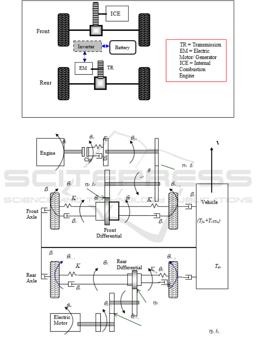
Figure 1: Schematic of the parallel powertrain architecture a 4WD of HEV.
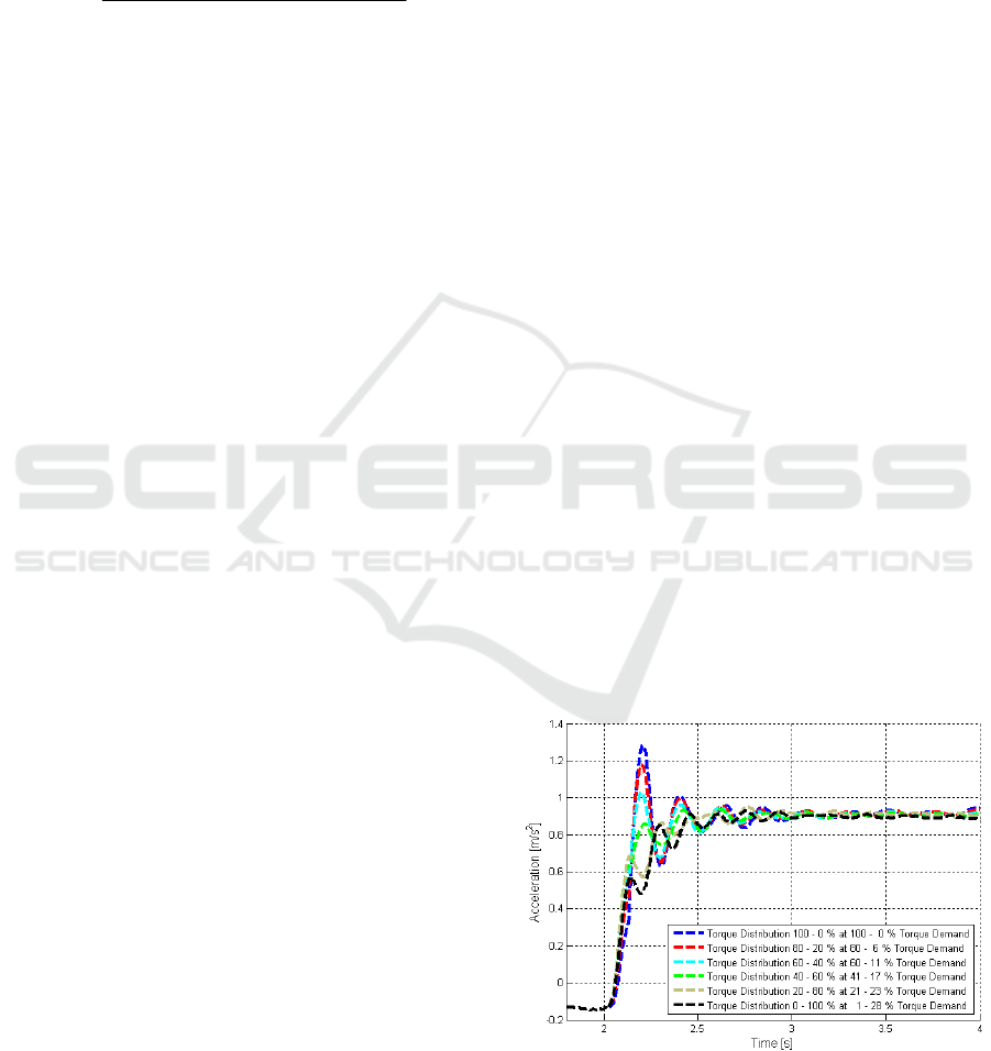
Figure 2: The schematic of the complex model of the 4WD HEV.
Dynamic Characteristic Evaluation of the Hybrid Electric Vehicle by Simulation
1441

• The longitudinal acceleration characteristic is
the main parameter which affects drivability
(Hohn and Stahl, 2011). Longitudinal
acceleration is associated with response delay,
overshoot, rise rate, jerk, and kick.
• Jerk (
kJ
) is the time rate of change in the
vehicle longitudinal acceleration
smX

. In
mathematical terms, jerk is defined as the
derivative of longitudinal acceleration and is
written as:
t
m
k
d
X
J
v

=
(1)
• Kick
)( kK
is the first decrease of longitudinal
acceleration. It can be expressed as:
min'1max1 ,, AAKk −=
(2)
Where
max,1A and min,1'A are the first peak
high and peak low overshoots.
• Rise time
)( rt
is the time required for the
response to rise from 10% to 90 % (rise rate) of
the steady-state value. This is the initial part of
vehicle response during gearshift or tip-in.
• Overshoot
)( vO the time required for the
response to settle within a certain range of the
steady-state is called the settling time.
2 MODELING DEVELOPMENT
OF THE FOUR-WHEEL-DRIVE
HYBRID ELECTRIC VEHICLE
The model will first be presented with a model
structure and detailed description of the mechanical
layout including governing equations. Mathematical
models that predict the vehicle dynamic
performances are created systematically in order to
evaluate the dynamic low frequency behavior. In
particular, the aim of the modeling is to determine
the most important dynamic physical parameters of
the vehicle that affect drivability during the
investigated transient conditions.
The studied model layout of the 4WD HEV is
depicted in Figure 2. The front powertrain in the
vehicle consists of an ICE coupled to a six speed
automated manual transmission through the friction
clutch. The output of the transmission drives the
front wheels through a pair of half-shafts. For the
rear powertrain, an EM is coupled to the rear axle
and drives the rear wheels through a two-speed
transmission integrated with the differential.
2.1 Engine Model
The engine is modeled through experimental maps,
which generate a theoretical engine torque as a
function of throttle position and engine speed. The
engine dynamics are determined through a first order
transfer function that depends on the engine
characteristic (e.g. time constant). The output of the
transfer function is the delayed torque (
deT
), which
is used for the moment balance equation of the
engine shaft.
For a body with constant moment inertia
rotating about a fixed axis, Newton’s second law of
motion is often referred that can be stated
mathematically according to:

=−
i
ext JT
i
0 θ

(3)
Where the summation over
i
includes all
torques acting on the body (
extT
);
J
is the moment
of inertia and
θ

is the angular acceleration.
Based on Newton’s law, the sum of the torques
acting on the engine and the clutch is satisfied by the
following equation:
eeecde JTT θ

=−
(4)
Where
deT
is the delayed engine torque and
ecT
is the engine clutch torque damper,
eJ
is the engine
moment inertia including the fly-wheel moment of
inertia, and
e θ

is the angular acceleration of the
engine.
Engine Gearbox Model
Primary shaft: The damping of the system
transmission of the gear box may be neglected
altogether (Cavallino and Turner, 2009).
The primary shaft torque is determined as:
111 ggecg JTT θ

−=
(5)
where
1gT
and
1gJ
are the primary shaft torque at
the front transmission and the inertia of the primary
shaft respectively;
1g θ

is the angular acceleration of
the primary shaft of the front transmission.
Secondary shaft: With the front driven axle, the
gear on the secondary shaft is connected to the
differential directly without using a propeller shaft
as shown in Figure 2. The gearbox losses (caused by
the internal friction) are represented by the lumped
efficiency
)(
f
g
η
The secondary shaft torque is determined:
iCAST-ES 2021 - International Conference on Applied Science and Technology on Engineering Science
1442

222
,
ggdg JTT
if
θ

+=
(6)
Where
if
dT
,
is the input shaft torque of the front
differential and
2g
T
is the secondary shaft torque,
2g
J
is the moment inertia of the secondary shaft and
2g θ

is the secondary shaft angular acceleration.
Differential and Drive Shaft Model: In the same way
as the gearbox transmission, the differential is
characterized by a gear ratio. The relation of the
differential input and output torque is simply
determined by considering the differential
conversion ratio and efficiency which is given,
ffiff
dddd iTT
η
,0,
=
(7)
Where
0,f
dT
is the output torque of the front
differential
f
di
is the front gear differential ratio and
f
d
η
is the differential efficiency. The differential
loss
The differential output torque is transmitted by
two different shafts (right and left shaft), each of
which is connected to the wheel through the half-
shafts. Since the right half-shaft is asymmetrical
with the left half-shaft (the right and the left
properties are not the caused by the internal friction)
is represented by the lumped efficiency.
The differential output torque is transmitted by
two different shafts (right and left shaft), each of
which is connected to the wheel through the half-
shafts. Since the right half-shaft is asymmetrical
with the left half-shaft (the right and the left
properties not the same), the torque balances on the
differential and half-shafts are expressed as:
𝑇𝑑
,
𝜂𝑑

𝑖𝑑

−𝑇𝑠
,
−𝑇𝑠
,
=[𝐽𝑑

+0.5(𝐽𝑠
,
+𝐽𝑠
,
)]𝜃

𝑑

(8)
Where
f
d θ

is the differential angular
acceleration,
Rf
sT
,
and
Lf
sT
,
are the right and left
half-shaft torque,
f
dJ
,
Rf
sJ
,
,
Lf
sJ
,
are the moment
inertia of the differential, the right and left half-
shaft, respectively.
1. Front Tyre Model: The wheel model is
characterized as a non-linear model. In this
case, the longitudinal traction forces (
xF
) are
modeled by using the Pacejka’s Magic Formula
(Pacejka, 2006).
The moment balance on the half-shaft to the wheel is
required in order to find the wheel angular
acceleration which is derived in the following
equation.
RfRfRfRfRfRf
wswrollws JJTTT
,,,,,,
)( θ

+=−−
(9)
Where,
Rf
wT
,
is the right front wheel torque and
Rf
wJ
,
is the tyre moment inertia.
The wheel torque performance is the function of
the longitudinal traction force (
xF
) and wheel
radius (
wR
). Hence, the tyre traction torque can be
written as:
wxw RFT
R
f
=
,
(10)
Rf
rollT
,
is the right front tyre rolling resistance torque
non-linear model, which is expressed as:
)(
2
3
,
2
,
10
, RfRfRf
wrwrrwvroll cccRwT θθ

++=
(11)
where
0rc
is the coefficient of the tyre,
1 rc
is the
coefficient of tyre pressure,
2rc
is the rolling
resistance coefficient depending on vehicle velocity
square, and
vw
is the vertical load for each wheel.
2.2 Electric Motor Axle Drivetrain
Model
The electric motor rear axle is modeled as a two-
speed gear. Due to the absence of a clutch damper,
the rear powertrain is a one degree of freedom
system in conditions of constant gear and two
degrees of freedom when the internal dynamics of
the differential gear set are considered.
2. Electric Motor Model: The EM is modeled in a
similar way to the engine model which is found
experimentally attained maps that generate a
theoretical motor torque as a function of the
pedal position and motor speed. The EM
dynamics are also determined through a first
order transfer function that depends on motor
dynamics. The output of the transfer function is
the delayed motor torque (
mT
).
The Electric Motor Transmission System:
The transmission utilizes a seamless shift system.
There are two kinds of clutch to provide a smooth
shifting man oeuvre; 1) a one-way sprag clutch for
transferring torque to the first gear, and 2) a friction
clutch to deliver torque to the second gear. On the
sprag clutch, there is a locking ring device, which
can prevent the one-way sprag clutch from
overrunning when the direction of torque through
Dynamic Characteristic Evaluation of the Hybrid Electric Vehicle by Simulation
1443

the transmission is reversed in order to allow
regenerative energy recovery whilst decelerating in
first gear (Holdstock et.al 2012). The clutch is
electro-hydraulically controlled through the use of a
remote brushless motor driven actuator, pressurizing
a master cylinder mechanically connected to the
Belleville spring of the friction clutch (Alcantar and
Assadian 2019). The moment balance equations of
the transmission shafts differ for each selected gear
due to the effect of the moment of inertia of the two
clutches mounted in the different shafts. Therefore,
the derivation for first gear and second gear dynamic
equations are determined in a different manner. The
first gear: when the clutch is engaged, the motor
torque will be transferred to the primary shaft. In
this condition, the sprag clutch engages while the
friction clutch disengages. The torque balance
equation for the first gear on the primary shaft which
is subjected to the motor torque is:
11)( gmmfcm TJJTT −++= θ

(12)
where
mT
is the motor torque and fcT the motor
friction clutch torque,
1gT is the primary shaft
torque, J
m
is the moment of inertia of the motor, J
1
the moment of inertia of the primary shaft, and
m θ

is
the angular acceleration of the motor.
The second gear: The moment balance equation
forthe primary shaft (in secondary gear selected) is
expressed as:
1211 )( ggmmbm TTJJJT ++++= θ

(13)
Where,
2gT
is the torque through the second
gear and
bJ1
is the moment of inertia of clutch.
3. Gear Box and Differential Model:
The moment balance equations of the transmission
shafts differ for each selected gear, therefore the
derived differential accelerations in gear one and
two are given below.
The first gear: The moment balance equation for
the primary shaft is given:
222222111 )( θηη

bdgg JJTiTiT
r
+=−+
(14)
bbfcg JTT 112 θ

−=
(15)
221 ib θθ

=
(16)
222 iJTT ibfcg θ

−=
(17)
where T
g1
and T
g2
are the primary and secondary
shaft torque,
fcT is the friction clutch torque,
r
dT
is
the differential torque,
bJ1
and
bJ2
are the moment
of inertia friction clutch and sprag clutch,
2J
is the
moment of inertia of the secondary shaft,
1i
and
2i
are the gear ratios for the first and second gears,
b1 θ

is the angular acceleration of the friction clutch and
2 θ

is the angular acceleration of the secondary
shaft,
1
η
and
2
η
are the first and the second gear
efficiencies. Combining eq. (14) and eq.(17), it gives
a form
𝑇𝑔1𝑖1𝜂1 + 𝑇𝑓𝑐𝑖2𝜂2 − 𝐽𝑖𝑏𝜃

2𝑖2

𝜂2 − 𝑇𝑑

=(𝐽2+𝐽2𝑏)𝜃

2 (18)
Where
12 /im θθ

=
and
𝑇𝑔1𝑖1𝜂1 − 𝑇𝑑

+ 𝑇𝑓𝑐𝑖2𝜂2 − 𝐽1𝑏𝜃

2𝑖2

𝜂2
= (𝐽2 + 𝐽2𝑏)𝜃

𝑑

𝑖𝑑

(19)
Substituting equation will give the result as
𝑇𝑑

=𝑇𝑚−𝑇𝑓𝑐−
(
𝐽𝑚 + 𝑗1
)
𝜃

𝑑

𝑖𝑑

𝑖1𝑖1𝜂1 +
𝑇𝑓𝑐𝑖2𝜂2 − 𝐽1𝑏𝜃

1𝑏𝑖2𝜂2−(𝐽2+𝐽2𝑏)𝜃

𝑑

𝑖𝑑

(20)
where J
2
is the moment inertia of secondary
shaft, i
1
and i
2
are the transmission ratio of the first
and secondary gear.
2.3 Chassis Model
For ride analysis, it is necessary to consider the
wheel and suspension as a lumped mass (namely
unsprung mass), whilst the vehicle body (sprung
mass) is another lumped mass. The sprung mass
governing equations (longitudinal displacement,
vertical displacement and pitch angle) will be
described initially, followed by the unsprung mass
governing equations (vertical displacement of the
unsprung mass and dynamic load transfer).
Sprung Mass Model:
For single mass representation, the vehicle body is
assumed as a mass concentrated at its centre of
gravity (
sm
G
). The point mass at the centre of
gravity, with appropriate rotational moments of
inertia, is dynamically equivalent to the vehicle body
itself for all motions in which it is reasonable to
assume the vehicle body to be rigid (Nizar and Mats
2017).
The aim of the model in this section is to analysis
the longitudinal acceleration, vehicle speed, vertical
displacement and pitch angle.
Longitudinal Force Balance for the Sprung Mass:
The longitudinal acceleration is found from the force
balance sprung mass equation. The external forces
resistances that affect the dynamic of the sprung
1ii
rr
ddm θθ

=
iCAST-ES 2021 - International Conference on Applied Science and Technology on Engineering Science
1444

mass are also included. The force balance is satisfied
by the equation,
0
,,,,
=−−−+++ incaersmsmjxjxjxjx FFXmFFFF
L
r
R
r
L
f
R
f

(21)
The longitudinal acceleration of the sprung mass is
expressed as:
sm
incaer
LRi
jx
LRi
jx
sm
m
FFFF
X
irif
−−+
=

== ,,
,,

(22)
where
f
jxF
and
r
jxF
are the front and rear traction
horizontal forces which from the tyres are
transmitted to the vehicle through the suspension
joints on the front and rear,
smm
is the mass of the
sprung mass,
smX

is the longitudinal acceleration of
the sprung mass,
aerF
and
incF
are the
aerodynamic drag and the inclination resistance
forces respectively. Subscript “R” and “L” denote
the right and left side of longitudinal traction forces.
The aerodynamic drag resistance force is
calculated as
22
5.0 wvdaaer RACF θρ

=
(23)
where
a
ρ
is air density,
dC
is the drag
coefficient, A is the vehicle cross section area,
v
θ

is
the vehicle angular velocity and
wR
is the wheel
radius. And the inclination resistance force is
calculated as,
ϕ
singMF vincl =
(24)
where
vM
is the vehicle mass,
g
is the gravity
acceleration and
ϕ
the road inclination. It is noted
that the longitudinal acceleration of the sprung mass
denoted as
smX

that is the vehicle longitudinal
acceleration. Hence, the jerk parameter of the
vehicle is equal to the derivative of the longitudinal
acceleration, equation (22).
3 SIMULATION RESULT
The sensitivity analysis is done by changing the
input parameters predicted to affect the vehicle
dynamic behavior during transient condition. The
parameters of the HEV powertrain such as the power
capacity of the power sources, the transmission gear
ratio, torque distribution and the capacity of battery
have significant influence on the vehicle
performance and operating efficiency (Kyoungcheol,
and Hyunsoo, 2017). These parameters will be taken
into account as inputs for the sensitivity analysis
with the exception of the capacity of battery. In the
case of the parallel 4WD HEV, the effect of varying
torque distribution is important when considering
the interaction of two powertrains to produce a
desired or undesired dynamic response.
In order to analyze the effect of torque
distribution for the vehicle dynamics response, all
combinations of the selected gear (front and rear
transmission) should be presented however, some of
the combinations can be represented by others as
their responsiveness trends are similar. Therefore,
only one combination of the selected gears are
chosen to be presented and evaluated. The front
transmission, first gear and rear transmission, second
gear
The torque distribution ratio was designed
starting from 100% ICE: 0% EM up to 0% ICE:
100% EM by decreasing the ICE by 20% and
increasing the EM by 20% at every step. Because
the overall value of wheel torque (the total torque
front and rear axles) remains the same, the torque
demand ratio for each certain torque distribution is
determined by the selected gear and the power
capacity of two powertrains.
The vehicle dynamic response parameters (as the
output of the sensitivity analysis) observed during
the tip-in test include the longitudinal acceleration,
jerk, speed, pitch angle and vertical displacement of
sprung mass.
Sensitivity Analysis:
In this case the vehicle was arranged to move with
the initial speed 19 km/h in the selected gear 1/2,
and then the tip-in test was performed with varying
torque distribution for sensitivity-analysis.
Figure 3: Sensitivity analysis of the longitudinal
acceleration during a tip-in test with the initial vehicle
speed 19 km/h and the selected gear 1/2.
Dynamic Characteristic Evaluation of the Hybrid Electric Vehicle by Simulation
1445

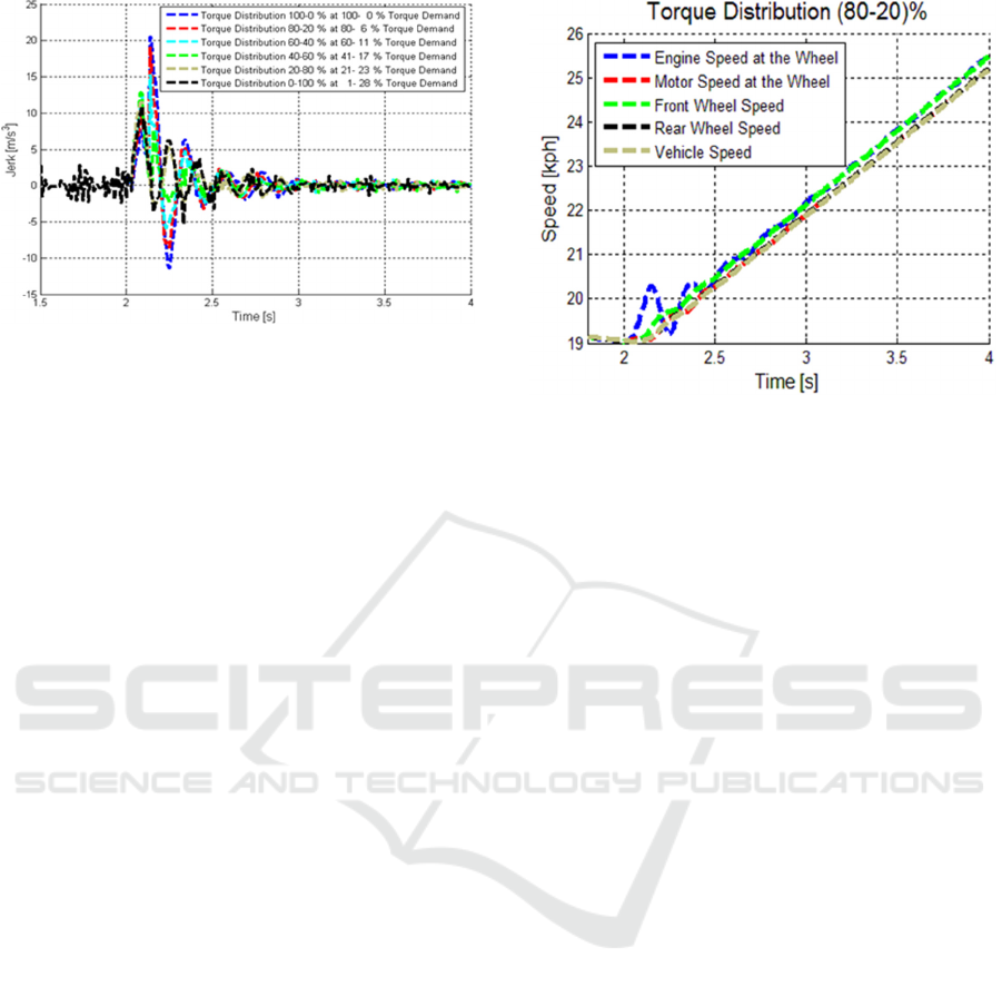
Figure 4: Sensitivity analysis of the jerk during a tip-in test
with the initial vehicle speed 19 km/h and the selected
gear 1/2.
Figure 3 shows varying responses of the vehicle
longitudinal accelerations. It shows an increase of
the acceleration oscillation for an increase of the
engine driven axle torque and torque demand. The
electric motor driven axle gives a small rise in
oscillation and low amplitude oscillation during this
test whilst the engine driven axle generates
significant high amplitude oscillation. It is shown in
Figure 3 that when the torque distribution of the EM
is dominant, the maximum torque demand is needed
only up to 28%. Figure 4 shows the jerk
characteristics with different torque distributions.
The results are similar to those for the acceleration.
The increased jerk oscillation values are obtained
when the engine torques are dominant compared to
the electric motor torque demand and vice versa.
The maximum jerk which can be reached when the
torque distribution 80% ICE: 20% EM is 20 m/s
3
whereas for the torque distribution 20% ICE: 80%
EM is approximately 12 m/s
3
. Figure 5 shows the
speed profiles for two manoeuvres where the torque
distribution on the front and rear is 80:20% ICE:EM,
and. The speed of different components at the wheel,
such as the engine and electric motor, are referred to
the vehicle speed (i.e. the engine speed is divided by
selected gear ratio and differential ratio and
multiplied by the wheel radius). As a consequence,
the figure shows the concurrent evaluation of the
torsion dynamics of both powertrain during the test.
Due to the initial torsion of the engine clutch
damper and the inside of the component, the speed
of the engine driven axle at the wheel tends to
oscillate before the first set of clutch springs starts to
transmit the torque. The simulation results show that
each couple of speeds (engine with front wheel speed
and motor with rear wheel speed) tends to converge
at the end of the transient condition when the half-
Figure 5: Speed comparison for each component speed
referred to the vehicle speed during a tip-in test with the
selected gear 1/2.
shaft reaches the steady-state torsion angle for that
value of transmitted torque. In both figures, the tyre
slip ratio dynamics are evident from the difference
between the vehicle speed and the respective wheel
speed. As a result of the transient condition, the
wheel speed profile is higher on the axle
transmitting the majority of the torque, the front axle
in Figure 4.
4 CONCLUSIONS
After the development of a model and following the
simulation, it is shown that the combination of the
torque characteristics of the ICE and the EM
propulsion and their transmission has the largest
impact on driveline responses, which affect
drivability. In addition, the vehicle dynamic
response behavior has high oscillations and a more
complex time history during hybrid mode due to the
combination of rapidly variable torque demand and
the first natural frequencies from two different
propulsions in transient condition.
ACKNOWLEDGEMENTS
I wish to thank to all my colloquies in the
Mechanical Department for involving during the
study. Thank to Director of the State Polytechnic
Ujung Pandang for providing facilities, and The
Higher Education Ministry of Indonesia (Direktorat
Riset dan Pengabdian Masyarakat, DRPM) for
supporting the research funding.
iCAST-ES 2021 - International Conference on Applied Science and Technology on Engineering Science
1446

REFERENCES
Giancarlo Genta and Lorenzo Morella, (2019). The
Automotive Chassis Volume 2: System Design, p 429,
Springer.
Liao, G. Y., Weber T. R. and Pfaff, D. P. (2004).
Modelling and Analysis of Powertrain Hybridization
on All-Wheel-drive Sport Utility Vehicles. Proceeding
Instn Mech. Engrs Vol. 218 Part D: Journal
Automobile Engineering.
Rizzoni, G., Guzzella, L., and Bernd, M. B. (2019).
Unified Modelling of Hybrid Electric Vehicle
Drivetrains. IEEE/ASME Transactions on
mechatronics. Vol. 4, No. 3.
Velazquez Alcantar J. & Assadian F. (2019). Vehicle
dynamics control of an electric-all-wheel- drive hybrid
electric vehicle using tyre force optimisation and
allocation, Vehicle System Dynamics, International
Journal of Vehicle Mechanics and Mobility, DOI:
10.1080/00423114.2019.1585556.
Hohn B. R., Stahl K., Pflaum H., and Draxal T. (2011).
Operating Experience with the Optimized CVT Hybrid
Driveline. Balkan Association of Power
Transmissions, Vol. 1, Issue 2, pp 32-38.
Cavallino C., and Turner A. (2009). Multi-Speed EV/FCV
Transmission with Seamless Gearshift. 8
th
International CTI Symposium, Innovative Automotive
Transmissions.
Pacejka, H. B. (2006). Tyre and vehicle dynamics.
Elsevier, 2nd Edition.
Holdstock T., Sorniotti A., Suryanto S., Leo S., Fabio V.,
and Carlo C. (2012). Linear and Nonlinear Methods to
Analyse the Drivability of a Trough the Road Parallel
Hybrid Electric Vehicle. International Journal of
Powertrain.
Nizar Chaar and Mats Berg (2017). Simulation of vehicle–
track interaction with flexible wheelsets, moving track
models and field tests, Vehicle System Dynamics:
International Journal of Vehicle Mechanics and
Mobility, DOI: 10.1080/00423110600907667.
Kyoungcheol O., Junhong M., Donghoon C., and Hyunsoo
K. (2017). Optimization of Control strategy for a
single-shaft parallel hybrid electric vehicle.
Proceeding IMechE Vol. 221 Part D: J. Automobile
Engineering, DOI: 10.1243/09544070JAUTO93.
Dynamic Characteristic Evaluation of the Hybrid Electric Vehicle by Simulation
1447