
Enhancement Accuracy of the Spatial Map Matching Algorithm using
Combine Test and Candidate Points in Mobile Application
Erika Vernanda
a
, Haniah Mahmudah
b
, Tri Budi Santoso, Okkie Puspitorini,
Nur Adi Siswandari and Ari Wijayanti
Electronics Engineering Polytechnic Institut of Surabaya, Sukolilo, Surabaya, Indonesia
ariw@pens.ac.id
Keywords: Map-Matching, GPS Position, Vehicle Trajectory.
Abstract: GPS often has errors in determining the position, causing the path shown to deviate from the proper route.
Can resolve the problems by using the map matching process. Map-matching is matching the GPS trajectory
between the GPS trajectory and the actual trajectory. The algorithm proposed to solve this problem is called
the Spatial Map-Matching Algorithm. Map-matching is used to map each raw GPS trajectory onto the road
network, which is always necessary and critical because GPS tracking data is inaccurate. The purpose of this
paper is to enhancement the performance of the Spatial Map-Matching Algorithm by selecting a number of
candidate points and test points on the Spatial Map-Matching Algorithm in order to find the best CMP value.
The combination of test points and selected candidate points can yield an optimal path that does not deviate
with a high degree of accuracy. As a result, the Spatial Map-Matching Algorithm can be used to solve map-
matching issues in GPS Smartphones.
1 INTRODUCTION
Smartphones are the most popular mobile devices
today equipped with GPS. Global Positioning
Systems (GPS) technology is using to obtain
positioning data. The integration of GPS is part of the
innovative advanced technology applied to
improving mobility and safety, reduce environmental
impacts, energy consumption, and enhance the
overall quality of life of individuals. When
integrating GPS measurements with a roadway
network in GIS, these measurements (represented as
data points) are usually projected to the nearest
roadway centerline segment to determine the road on
which events and incidents occur, point features are
locating, or a vehicle is traveling (Blazquez et al.,
2018).
The problem is often encountering when using
GPS is the position error of the GPS sensor, which
causes the point to be inaccurate. Besides that, other
factors affect the accuracy of the map-matching
algorithm, namely the complexity of the highway
a
https://orcid.org/0000-0003-0848-257X
b
https://orcid.org/0000-0002-1675-2077
network because ambiguous matching cases are more
likely to occur (Hsueh et al., 2018). In overcoming the
problem of position errors, you can use a technique
called map-matching. Map-matching handles the
problem of matching GPS trajectories with roads on
a digital map and deduces the actual position for each
sampling point to be supposed the Real route for the
entire sampling path (Hu et al., 2017).
Some examples of well-known map-matching
algorithms such as Interactive-Voting Based Map
Matching (IVMM) or commonly called Spatial Map-
Matching (Yuan et al., 2010), Hidden Markov Model
(HMM) (Hsueh et al., 2018), Ant Colony-Based Map
Matching (AntMapper) (Gong et al., 2018), and
Fuzzy Logic (Yongqiang Zhang & Gao, 2008).
Using the map-matching technique can handle
lower sampling rates and lower localization accuracy
(Mohamed et al., 2017). The advantages, there are
also challenges faced in map-matching, namely first,
to save energy and communication costs. Second, due
to sensor failure causes sampling data to be unusable
due to some missing data. Third, road-intensive
976
Vernanda, E., Mahmudah, H., Santoso, T., Puspitorini, O., Siswandari, N. and Wijayanti, A.
Enhancement Accuracy of the Spatial Map Matching Algorithm using Combine Test and Candidate Points in Mobile Application.
DOI: 10.5220/0010957500003260
In Proceedings of the 4th International Conference on Applied Science and Technology on Engineering Science (iCAST-ES 2021), pages 976-982
ISBN: 978-989-758-615-6; ISSN: 2975-8246
Copyright
c
2023 by SCITEPRESS – Science and Technology Publications, Lda. Under CC license (CC BY-NC-ND 4.0)

factors will also affect map-matching (Hsueh et al.,
2018).
This map-matching algorithm has been applying
to several location-based applications such as car
navigation, direction finding, car direction
estimation, automatic scheduling of public
transportation systems, traffic analysis, and so on
(Mohamed et al., 2017). Some studies that also apply
map-matching algorithm, such as low sampling rate
from GPS track (Hsueh et al., 2018), wheelchair
navigation (Ren & Karimi, 2012), Track Based
Applications (Gong et al., 2018), Bus Lane
Identification (Raymond & Imamichi, 2016).
Another study using the IVMM Algorithm
revealed that the weight of the distance is very
influential, while the weight of the sampling point has
an effect on the network topology of a road (Yuan et
al., 2010) and only observes the percentage of the
sampling rate.
The weakness of a previous study titled “An
Interactive-Voting Based Map Matching Algorithm"
(Yuan et al., 2010) is that it only refers to the
sampling interval. In the previous paper, two
algorithms, IVMM and ST-Matching, were
compared. When the sampling interval is between 1.5
and 6.5 minutes, the IVMM accuracy is always
around 70%, a 10% improvement over the ST-
Matching algorithm (Yuan et al., 2010), while the
Spatial Map-Matching Algorithm has a maximum
accuracy value of 100%. When processing data, this
algorithm has the advantage of producing a higher
matching accuracy value.
The purpose of this paper is to enhancement the
performance of the Spatial Map-Matching algorithm
by selecting number of candidate points and test
points on the Spatial Map-Matching Algorithm in
order to find the best CMP value. The IVMM
algorithm considers the GPS trajectory's spatial and
temporal information and models the weighted
reciprocal effect between GPS points. However, the
IVMM algorithm process is complex, and the data
must be matched repeatedly. Furthermore, the
distance between the two sampling points of the
matched track is too great. Using the Spatial-Map
Matching algorithm, the distance between the two
sampling points of the track is not too great, it only
requires a distance of 50m between the two sampling
points. This algorithm measures the relationship
between successive candidate points in a map match
using the spatial analysis function and the ST-
function.
2 RELATED WORK
This section is a description of several Map-Matching
Algorithms that have developed. Reviewing the
description, methodology, and final results of the
algorithm used.
2.1 IVMM
Algorithm IVMM is an algorithm that is by far the
only approach aimed at GPS data with low sample
rates in terms of match quality.
The IVMM process works, namely the first
candidates preparation, the second position context
analysis, the third mutual influence modeling, divided
to 2 namely Static Score Matrix Building and Weight
Influence Modeling and Interactive Voting (Yuan et
al., 2010). The results obtained are four results. The
first result is virtualization. For the second result,
namely the results of the CMP calculation. Third, the
Running Time of the IVMM Algorithm is very high
speed for data with low sampling rates and high
sampling rates (Yuan et al., 2010).
2.2 Hidden Markov Model (HMM)
The HMM model is a statistical model that has the
challenge of determining the hidden parameters
(state) of the observable parameters (observer). Map-
Matching algorithm that uses HMM modeling is
called STD-Matching. In the STD-Matching process,
there are three processes, namely Extraction of
Candidate Set Extractions, STD Analysis, and
Matched Answer Computation (Hsueh et al., 2018).
STD Analysis, three pieces of information would be
considered, namely spatial, temporal and directional
information. The advantage of the STD-Matching
Algorithm is that it produces superior matching
accuracy values in high sampling and low sampling
rates (Hsueh et al., 2018).
2.3 Ant Colony-based Map Matching
(AntMapper)
The process of AntMapper consists of 3 processes,
firstly applying transition rules. The second is to
update pheromones, which are, carried out globally
and locally. The third is the termination process, by
starting a new round of path construction repeatedly
until the termination rules are met (Gong et al., 2018).
The AntMapper Algorithm has the advantage that
it can find the underlying structure of the problem
space (Gong et al., 2018). But, have a limitation that
it cannot provide strong enough evidence to prove
Enhancement Accuracy of the Spatial Map Matching Algorithm using Combine Test and Candidate Points in Mobile Application
977
that it has strong capabilities in various application
fields such as global optimization capabilities.
The results are using the AntMapper Algorithm
can be seen from two sides, namely Synthetic
Instances, and Real-Life Instances.
2.4 Fuzzy Logic
The technique used in this map-matching algorithm is
called Fuzzy Logic, where this technique is usually
used to solve very complicated systems and is the
correct technique in mapping an input space to an
output space. There are three steps to process this
technique, the first, to perform input and output
fuzzification, the second, to build the rule base, and
the last is to defuzzify the output (Yongqiang Zhang
& Gao, 2008). By using Fuzzy Logic, it can have
much higher precision.
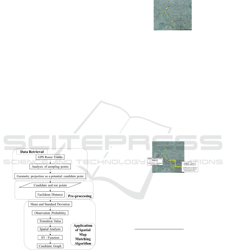
3 METHODOLOGY
The methodology used in the Spatial Map Match
Algorithm is described in this section. It is divided
into three stages: data retrieval, pre-processing, and
use of the Spatial Map Matching Algorithm. Figure 1
shows the methodology's flowchart.
Figure 1: Methodology’s Flowchart.
3.1 Data Retrieval
Before taking data, it is better to digitize the route
first. Determine which road to take, then determine
specific points on the right or left side of the road.
Data retrieval already completed using a GPS
Smartphone. Figure 2 is an example of Digitizing
Routes.
Figure 2: Route Digitization.
3.2 Pre-processing
Pre-processing is the initial process in calculating the
Spatial Map-Matching Algorithm, which is to prepare
the data that already used for further calculations. The
data need to be prepare, the candidate points search
and euclidean distance.
Candidate points is available from digitizing the
previous route. This point is a point that shows the
actual path of the road. Unlike the test points, it is a
point that deviates from the road route. There are
three processes in the search for candidate points,
namely the first to find the road trajectory on the GPS.
Second, analyze the sampling point. Third, perform
Geometry projections as candidate points. Figure 3 is
a description of the search for candidate points.
Figure 3: Candidate Point Search.
Euclidean distance method is a method of
finding the proximity of the distance of 2 variables.
In this case, the two variables are the distance
between the test and candidate points, which is then
converted to one degree of the earth. By employing
Equation (1):
𝑥
−𝑥
𝑦
−𝑦
𝑥 111,319
(1
)
where 𝑥
, 𝑥
is 𝑥-coordinate, 𝑦
𝑦
is 𝑦-coordinate and
111,319 is 1 degree of the earth.
3.3 Application of Spatial Map
Matching Algorithm
The following step is implementation. Where the
collected data is processed for the next calculation. In
this process, the main step of the Spatial Map-
iCAST-ES 2021 - International Conference on Applied Science and Technology on Engineering Science
978

Matching Algorithm has begun. The Spatial Map-
Matching Algorithm is implemented in three steps:
the first is calculating the observation probability and
transition value, the second is calculating the spatial
and ST-function analysis, and the third is creating a
candidate graph.
The observation probability and transition value
are calculated first. Observation probability has been
using to determine the level of matching between test
points and candidate points. If the candidate points is
far from the test points, then the probability level of
matching the test points with the candidate points is
lower. Otherwise, the matching rate may be higher.
Calculating the observation probability data requires
euclidean distance, mean and standard deviation. In
equation (2), the following calculation is used to find
the mean:
𝑀𝑒𝑎𝑛
∑
𝑥
𝑛
(2)
where
∑
𝑥
is total of all data values and 𝑛 is
amount of data
In terms of calculating the standard deviation using
equation (3):
𝑆𝑡𝑎𝑛𝑑𝑎𝑟𝑑 𝐷𝑒𝑣𝑖𝑎𝑡𝑖𝑜𝑛
∑
𝑥
−𝜇
𝑛−1
(3)
where 𝑥
is value of 𝑥 to 𝑖, 𝜇 is mean and 𝑛 is amount
of data
So, to calculating the observation probability, use
equation (4):
𝑁𝑐
1
√
2𝜋𝜎
𝑒
(4)
where 𝑥
is the euclid distance from candidate 𝑐
to
sampling point 𝑝
.
The test points can be fixed using the transition
value calculation. The primary use of the transition
value is used for calculations between the distance of
the previous closest candidate point to the next
candidate points and based on test points that are
close to each other. The calculate is by equation (5):
𝑉
𝑐
→𝑐
𝑑
→
𝑤
,→,
(5)
where 𝑑
→
is the euclid distance from sampling
point 𝑖−1 to sampling point 𝑖, and 𝑤
,→,
is
the length of the shortest path from candidate 𝑐
to
𝑐
.
The Spatial analysis and ST-function are the next
steps. The spatial analysis function serves as the
analysis of the similarity between the shortest path in
both point adjacent candidate and candidate paths.
The equation spatial analysis function is the product
of the results of the observation probability and the
transition value, such as equation (6):
𝐹
𝑐
→𝑐
𝑁𝑐
∗𝑉
𝑐
→𝑐
(6
)
where 𝑁𝑐
is observation probability and
𝑉
𝑐
→𝑐
is transition value.
ST-function aims to get the best answer suitable
for the GPS track. Later the path that matches the
highest overall score is considered the most suitable
answer. The equation, it's a combination of all the
results of the previous calculations by multiplying all
of them, as in equation (7):
𝐹
𝑐
→𝑐
𝑁𝑐
∗𝑉
𝑐
→𝑐
∗𝐹
𝑐
→𝑐
(7
)
where 𝑁𝑐
is observation probability, 𝑉
𝑐
→
𝑐
is transition value and 𝐹
is the spatial analysis
function.
The third step is to creating a candidate graph.
Where this candidate graph is employed to aid in the
matching process. This candidate points is available
from digitizing the previous route. This point is a
point that shows the actual path of the road. Unlike
the test points, it is a point that deviates from the road
route. There are three processes in the search for
candidate points, namely the first to find the road
trajectory on the GPS. Second, analyze the sampling
point. Third, perform geometry projections as
candidate points. Candidate graph is shown as in
Figure 4.
Figure 4: Candidate Graph.
4 EXPERIMENT & RESULT
This section is an experiment to evaluate the proposed
algorithm, namely Spatial Map-Matching. From the
test results will be able to find out the advantages or
disadvantages of this algorithm. From the results can
perform analysis through Correct Matching
Percentage (CMP) and Graphs.
Spatial Map-Matching Algorithm Testing is
divided into three scenarios. The first scenario
employs two test points, the second employs three,
Enhancement Accuracy of the Spatial Map Matching Algorithm using Combine Test and Candidate Points in Mobile Application
979
and the third employs four. Six candidate points are
combined on the three scenarios.
4.1 Combining Test and Candidate
Points for Testing
The first step before testing is called data collection,
and it determines the points to be tested and selected
the coordinates to be used. In addition, the Spatial
Map-Matching Algorithm implementation is carried
out. The results are displayed in a candidate graph and
the percentage of accuracy is calculated (CMP value).
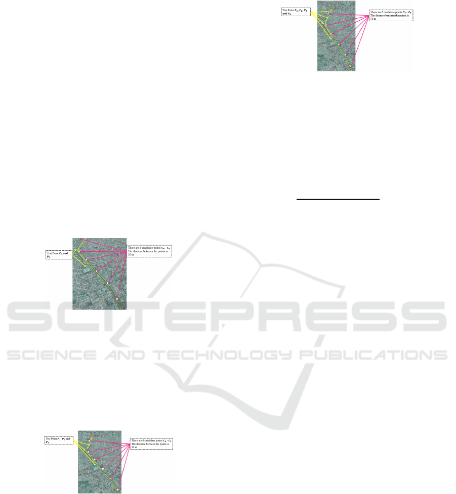
The first test scenario combines two test points
(𝑷
𝟏
dan 𝑷
𝟐
) and six candidate points ( 𝑪
𝟒
−𝑪
𝟗
).
Figure 5 shows that the two-test points appear to
deviate from the correct path. The candidate point is
located on the correct path. The most optimal path is
found at candidate points 𝑪
𝟓
and 𝑪
𝟕
as a result of the
first scenario.
Figure 5: Scenario I.
In the second test scenario, three test points
(𝑷
𝟏
, 𝑷
𝟐
dan 𝑷
𝟑
) and six candidate points (𝑪
𝟒
−𝑪
𝟗
)
are combined. The three-test points appear to deviate
from the correct path, as shown in Figure 6. The
candidate points is on the correct path. As a result of
the second scenario, the most optimal path is found at
candidate points 𝑪
𝟓
, 𝑪
𝟔
, and 𝑪
𝟗
.
Figure 6: Scenario II.
The third test scenario integrates four test points
(𝑷
𝟏
, 𝑷
𝟐
, 𝑷
𝟑
dan 𝑷
𝟒
) and six candidate points (𝑪
𝟒
−
𝑪
𝟗
). The four- test points appear to deviate from the
correct path, as shown in Figure 7. The candidate
points is on the correct path. As a result of the third
scenario, the most optimal path is found at candidate
points 𝑪
𝟒
, 𝑪
𝟓
, 𝑪
𝟕
, and 𝑪
𝟗
.
Figure 7: Scenario III.
After the scenario parameters are determined then
the calculation of system performance using
Calculation Correct Matching Percentage (CMP).
The CMP is used by the Spatial Map-Matching
Algorithm to determine the accuracy of the algorithm
and to evaluate the quality of the match, such as
equation (8):
𝐶𝑀𝑃=
x 100%
(8
)
4.2 Testing Graph
In the test scenario, the Mean and Standard Deviation
are 0.32 and 0.2; 5 and 10; 50 and 10 are then
calculated. The first step is to calculate the euclidean
distance between the test and candidate points using
the formula in equation 1, then calculate the mean
using the data from the euclidean distance
calculation, using the formula in equation 2. For the
calculation formula in equation 3, the mean results
will be used to calculate the standard deviation. Using
the formula in equation 4, these three data, namely
euclidean distance, mean, and standard deviation, will
be used to calculate the probability of observation.
The transition value is then calculated using the
formula in equation 5. To calculate Spatial Analysis,
the results of the two data sets will be multiplied as in
equation 6. After obtaining the three data points, use
the formula in equation 7 to compute the ST-function.
After all calculations have been completed, create a
candidate graph, as shown in Figure 3, to aid in the
matching process. The number of correct candidate
points, as well as the candidate points that represent
the most optimal path, will be determined by the
results of the candidate graph. Following that, a CMP
calculation will be performed to determine the level
of accuracy, which will be determined by dividing the
number of correct candidate points by the number of
points to be matched, as shown in equation 8. A graph
is created to compare the test results when different
combinations of mean and standard deviation are
used. as shown in Figures 8, Figures 9, and Figures
10.
Figure 8 depicts the graphical results of the first
scenario. The highest CMP scores are found in 2
iCAST-ES 2021 - International Conference on Applied Science and Technology on Engineering Science
980
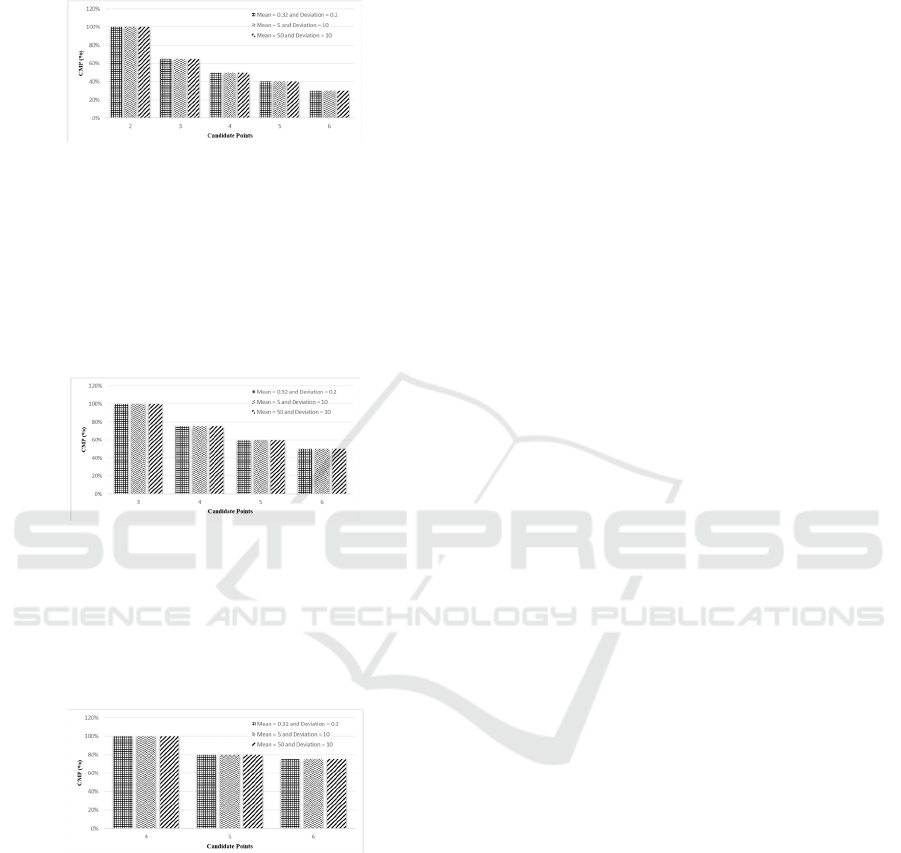
candidate points, with a perfect score of 100 percent,
and for the use of other candidate points, they are
around 75%, 50%, 40%, and 30%, respectively.
Figure 8: Scenario Graph I.
Figure 9 depicts the graphical results of the second
scenario. The highest CMP value is found in two
candidate points that both have a perfect score of 100
percent. There is only one chart, namely at 6
candidate points, where the CMP value is correct at
50%, while the others are above 50%, namely 60%
and 75%.
Figure 9: Scenario Graph II.
Figure 10 depicts the graphical outcome of the
third scenario. With a perfect score of 100 percent,
the highest CMP score is 4 candidate points. And in
all 3 scenarios, the CMP value is greater than 50%,
with the lowest CMP value being 70%.
Figure 10: Scenario Graph III.
Can saw from the results in the form of graphs, in
Figure 7 it's that by using two candidate points, the
percent accuracy value increases very significantly so
that it achieves a perfect score while using 3 to 6
candidate points. The percentage of accuracy value
decreases along with the increasing number of
candidate points used. Figure 8 also experienced
similar things the increased the number of candidate
points has been using, the smaller the value of
accuracy.
In addition, the test points used also affect the
candidate points as shown in the graph, when, using
2 test points, the maximum number of candidate
points used can be up to 6 candidate points, while 3
test points can only use a maximum of 5 candidate
points. And so also when using 4 test points can only
four candidate points. The more test points, the lower
the maximum number of candidate points that can
use. The number of test points and candidate points
affects the computational performance of the
algorithm.
5 CONCLUSIONS
In this paper, we can solve the problem of matching
maps on GPS Smartphones to improve route accuracy
by selecting a number of candidate points and test
points. The test point data is obtained from real-time
GPS data from the smartphone, which is then
processed. The calculation of the mean and standard
deviation has no effect on the level of route accuracy,
which is influenced by the number of candidate points
and test points. When only two candidate points are
selected, the results obtained by using the mean and
standard deviation of the calculations, namely 0.32
and 0.2; 5 and 10; 50 and 10 have the same level of
accuracy, namely 100%. The level of accuracy will
be lower if a larger number of candidate points are
chosen with the same combination of mean and
standard deviation. According to the test results, the
accuracy obtained by selecting the most candidate
points, namely 6 candidate points, is very low,
ranging from 50% to less than 50%. If more test
points and candidate points are chosen from the three
scenarios, the accuracy level will be lower and it will
be more difficult to find the most optimum path due
to the low level of accuracy obtained.
REFERENCES
Blazquez, C., Ries, J., Miranda, P. A., & Leon, R. J. (2018).
An Instance-Specific Parameter Tuning Approach
Using Fuzzy Logic for a Post-Processing Topological
Map-Matching Algorithm. IEEE Intelligent
Transportation Systems Magazine, 10(4), 87–97.
Hsueh, Y. L., Chen, H. C., & Huang, W. J. (2018). A
Hidden Markov Model-Based Map-Matching
Approach for Low-Sampling-Rate GPS Trajectories.
Proceedings - 2017 IEEE 7th International Symposium
on Cloud and Service Computing, SC2 2017, 2018-
Janua, 271–274.
Hu, G., Shao, J., Liu, F., Wang, Y., & Shen, H. T. (2017).
IF-Matching: Towards accurate map-matching with
Enhancement Accuracy of the Spatial Map Matching Algorithm using Combine Test and Candidate Points in Mobile Application
981

information fusion. Proceedings - International
Conference on Data Engineering, 9–10.
Mohamed, R., Aly, H., & Youssef, M. (2017). Accurate
Real-Time Map Matching for Challenging
Environments. IEEE Transactions on Intelligent
Transportation Systems, 18(4), 847–857.
Ren, M., & Karimi, H. A. (2012). A fuzzy logic map
matching for wheelchair navigation. GPS Solutions,
16(3), 273–282.
Zhang, Yaying, & He, Y. (2018). An advanced interactive-
voting based map matching algorithm for low-
sampling-rate GPS data. ICNSC 2018 - 15th IEEE
International Conference on Networking, Sensing and
Control, 2, 1–7.
Raymond, R., & Imamichi, T. (2016). Bus trajectory
identification by map-matching. Proceedings -
International Conference on Pattern Recognition, 0,
1618–1623.
Yuan, J., Zheng, Y., Zhang, C., Xie, X., & Sun, G. Z.
(2010). An Interactive-Voting based Map Matching
algorithm. Proceedings - IEEE International
Conference on Mobile Data Management, 43–52.
Gong, Y. J., Chen, E., Zhang, X., Ni, L. M., & Zhang, J.
(2018). AntMapper: An Ant Colony-Based Map
Matching Approach for Trajectory-Based Applications.
IEEE Transactions on Intelligent Transportation
Systems, 19(2), 390–401.
Zhang, Yongqiang, & Gao, Y. (2008). A fuzzy logic map
matching algorithm. Proceedings - 5th International
Conference on Fuzzy Systems and Knowledge
Discovery, FSKD 2008, 3, 132–136.
Ma, C., Zhang, X., Gao, P., Dong, W., & Li, C. (2016).
Space-map-matching-based candidate selection for
GPS map matching. Proceedings - 2016 IEEE
International Conference on Service Operations and
Logistics, and Informatics, SOLI 2016, 77–82.
iCAST-ES 2021 - International Conference on Applied Science and Technology on Engineering Science
982
