ARIMA Modeling for Prediction of Inorganic Chemical Pollution in

the Kalitambong Watershed, Bondowoso Regency

Rizza Wijaya

and Budi Hariono

Department of Agriculture Engineering, Politeknik Negeri Jember, Jl Mastrip PoBox 164, Jember, Indonesia

Department of Food Engineering Technology, Politeknik Negeri Jember, Jl Mastrip PoBox 164, Jember, Indonesia

Keywords: Kalitambong Watershed, Contamination, ARIMA.

Abstract: T DAS (Watershed Area) is a part of land that includes rivers and their derivatives which function as storage,

reservoirs, and one of the media for the flow of water from rain to lakes and seas. The Kalitambong watershed

is included in the Bondowoso Regency, East Java. Kalitambong watershed is located on the border of

Bondowoso Regency and Banyuwangi Regency, precisely in Kabat District which has an area of

184,779,139.38 m2 or 184,779 km2. This research was conducted to predict the contamination contained in

the Kalitambong watershed, especially on the parameters of chemical-inorganic contamination with ARIMA

model. The result of this study is that the best ARIMA model for ARIMA pH parameter (3,0,0) with AIC

value of 51.63 and RMSE 0.581. The best model BOD parameter is ARIMA (2,0,0) with AIC value of 42.7

and RMSE 2.928. The best model COD parameter is ARIMA (0,2,1) with AIC of 34.7 and RMSE .,918. The

DO parameters of the best model are ARIMA (0,1,0) with AIC and RMSE of 13.24 and 0.46. Total phosphate

parameters with ARIMA model (0,1,0) with AIC value of 42.7 and RMSE of 2.92.

1 INTRODUCTION

The Kalitambong watershed is included in the

Bondowoso Regency, East Java. The Water

Resources Management Center (BPSDA) of

Bondowoso Regency has 10 watershed areas,

including Kalitambong watershed, Sampean

watershed, Deluwang watershed, Lobawang

watershed, Tlogo watershed, Curahmacan watershed,

Kalibaru watershed, Stail watershed, Bomo

watershed and Bajulmati watershed. Kalitambong

watershed is located on the border of Bondowoso

Regency and Banyuwangi Regency, precisely in

Kabat District which has an area of 184,779,139.38

m2 or 184,779 km2 and geographical coordinates are

located 8֯ 16' 54.32" South Latitude and 114 18'

59.34" East Longitude (Sugiyarto, Hariono, Wijaya,

Destarianto, & Novawan, 2018).

DAS (Watershed Area) is a part of land that

includes rivers and their derivatives which function as

storage, reservoirs, and one of the media for the flow

of water from rain to lakes and seas. The land part is

a topographical distinction and the sea boundary to

the water area that is still affected by land activities.

In a watershed ecosystem there are various processes

of interaction between various components, namely

soil, water, vegetation and humans. The river as the

main component of the watershed has a balanced

potential shown by the river's usability, among others,

for agriculture and energy. However, rivers can also

have a negative impact on the environment, including

overflowing river water that can cause flooding,

carriers of sedimentation, carriers of waste (Black,

1996).

Water is an important environmental component

for life and good life for humans, flora, fauna and

living things other. At this time water is a problem

that needs serious attention. To get good water

according to certain standards, it is now an expensive

item because water has been polluted by various

kinds of waste from various human activities. So that

in terms of quality, water resources have decreased.

Likewise in terms of quantity, which is no longer able

to meet the growing needs. The main problems of

water resources include the quantity of water that is

no longer able to meet the increasing human needs

and the quality of water for domestic purposes

continues to decline, especially for drinking water (Li

et al., 2018). As a source of community drinking

water, it must fulfill several aspects including

quantity, quality and continuity. Water quality is a

term that describes the suitability or suitability of

102

Wijaya, R. and Hariono, B.

ARIMA Modeling for Prediction of Inorganic Chemical Pollution in the Kalitambong Watershed, Bondowoso Regency.

DOI: 10.5220/0010940700003260

In Proceedings of the 4th International Conference on Applied Science and Technology on Engineering Science (iCAST-ES 2021), pages 102-108

ISBN: 978-989-758-615-6; ISSN: 2975-8246

 2023 by SCITEPRESS – Science and Technology Publications, Lda. Under CC license (CC BY-NC-ND 4.0)

water for certain uses, for example: drinking water,

fisheries, irrigation/irrigation, industry, recreation

and so on. Caring for water quality is knowing the

condition of water to ensure safety and sustainability

in its use. Water quality can be known by performing

certain tests on the water (Shrestha & Wang, 2020).

Most cities in developing countries discharge 80-

90% of untreated wastewater directly into rivers

where the river water is then used for drinking,

bathing and washing purposes (Taloor et al., 2020).

Disposal of industrial and household wastewater

causes river pollution in India, China, Latin America

and Africa . In Indonesia, almost most of the rivers in

Indonesia have been polluted, the status of river

quality in 2008 of 30 rivers in Indonesia, 86% have

been polluted from mild to severe.Water quality is the

nature of water and the content of living things,

energy substances or other components in the water.

Water quality is expressed by several parameters,

namely physical parameters such as: Total Dissolved

Solids (TDS), Total Suspended Solids (TSS), and so

on), chemical parameters (pH, Dissolved Oxygen

(DO), BOD, metal content and so on), and parameters

biology (Content of Coliform Bacteria, E-coli,

presence of plankton, and others). Measurement of

water quality can be done in two ways, the first is

measuring water quality with physical and chemical

parameters, while the second is measuring water

quality with biological parameters (B Hariono,

Wijaya, Kurnianto, Wibowo, & Anwar, 2018). This

research was conducted to predict the contamination

contained in the Kalitambong watershed, especially

on the parameters of chemical-inorganic

contamination. ARIMA (Autoregressive Integrated

Moving Average) model was developed by George

Box and Gwilyn Jenkins. This method is very good

for short-term predictions, and is not recommended

for long-term predictions because the results of the

prediction accuracy are not good. ARIMA is a

method that uses past and present data as the

dependent variable to produce accurate short-term

predictions.

2 METHODS

This research was conducted in the Kalitambong

watershed in collaboration with the BPSDA of

Bondowoso Regency. The data obtained in the form

of inorganic chemical contamination from January to

December 2017. The data inorganic chemical

contamination is pH, BOD, COD, DO, Total Fosfat

and NO3-N. Data analysis using the ARIMA method

was carried out using the R-Studio software.

2.1 ARIMA (Autoregressive Integrated

Moving Average

ARIMA is a stochastic method that is very useful for

generating time series processes (data) where each

event is correlated. ARIMA is very strict on

assumptions (data and residual white noise) and is

used for data with linear patterns. Literally, the

ARIMA model is a combination of the AR

(Autoregressive) model and the MA (Moving

Average) model. The ARIMA model consists of three

basic steps, namely the identification stage, the

assessment and testing stage, and the diagnostic

examination. Furthermore, the ARIMA model can be

used to make predictions if the model obtained is

adequate. ARIMA (Box-Jenkins) model is

formulated with ARIMA notation (p, d, q) (Siami-

Namini, Tavakoli, & Namin, 2018):

p: Indicates the order/degree of Autoregressive (AR)

d: Indicates the order/degree of Differencing

(distinction)

q: Shows the order/degree of Moving Average (MA)

2.2 Autoregresif Model

(Autoregressive)

Autoregressive model is a model whose dependent

variable is influenced by the dependent variable itself

in previous periods and times. In general, the

autoregressive (AR) model with the order p (AR(p))

or the ARIMA model (p,0,0) has the following form:

Yt = φ0+φ1Yt-1 + φ2Yt-2+ … +φpYt-p +et , (1)

where:

Yt : stationary time series Yt-1, Yt-2,….,, Yt-p =

Variable response to each time interval t - 1, t -

2,…, t - p. The value of Y acts as an independent

variable.

φ : Constant

φp : p-th autoregressive parameter

: Error at time t which represents the impact of

variables not explained by the model.

From the AR model (which is given the notation

p) is determined by the number of periods of the

dependent variable included in the model.

2.3 MA Model (Moving Average)

The moving average model of the order q (MA (q))

or ARIMA (0,0, q) has the following form:

Yt = θ0+et - θ1et-1 - θ2et-2 - … -θpet-q, (2)

ARIMA Modeling for Prediction of Inorganic Chemical Pollution in the Kalitambong Watershed, Bondowoso Regency

103

where

Yt: Stationary time series

θ0: Constant

θ1,…,θq: Parameters moving average which shows

the weight.

et – q: Error value at time t – k

2.4 ARMA Model (Autoregressive

Moving Average)

The model that contains both AR and MA processes

is called the ARMA model. The general form of this

model is:

𝑌𝑡 = 𝛾0 + 𝜕1𝑌𝑡−1 + 𝜕2𝑌𝑡−2 + ⋯ + 𝜕𝑛𝑌𝑡−𝑃 −

𝜆1𝑒𝑡−1 −

𝜆

2𝑒𝑡−2 − 𝜆𝑛𝑒𝑡−𝑞

(3)

where Yt is the stationary time series and et is the

error. If the model uses two dependent lags and three

residual lags, the model is denoted by ARMA. And if

you add a data stationary process, the existing ARMA

model becomes the general ARIMA model (p,d,q).

2.4 Forecasting

At this stage, a suitable model is found, but not the

actual model because there are still errors in it. The

forecast results are said to be good if they have a small

error rate, meaning that the forecast value is close to

the actual value. The following are the criteria for

selecting the best model before forecasting:

2.4.1 AIC (Akaike Information Criterion)

A criterion for selecting the best model that considers

the number of parameters in the model. AIC criteria

can be formulated as follows:

AIC = n ln (𝜎̂𝜀 2 ) + 2(𝑝 + 𝑞 + 1), 𝜎̂𝜀 2 (4)

2.4.2 SBC (Schwart’s Bayesian Criterion)

Criterion for selecting the best model based on the

smallest value. SBC criteria can be formulated as

follows:

SBC = n ln (𝜎̂𝜀 2 ) + 2(𝑝 + 𝑞 + 1) ln 𝑛

(5)

3 RESULTS AND DISCUSSION

This study used are inorganic chemical contamination

data, namely pH, BOD (Biological Oxygen Demand),

COD (Chemical Oxygen Demand), DO (Dissolved

Oxygen), Total Phosphate and NH3-N data from

January - December 2017. Monthly data January to

September is used to create and test the forecasting

model using actual data in October – December 2017.

Inorganic chemical contamination Kalitambong

watershed data can be seen in Table 1. Table 1 shows

that the contamination in the Kalitambong watershed

is classified as quality standard status 3, which means

that it is classified as a moderate level of

contamination (Budi Hariono, Wijaya, Anwar, &

Wahyono, 2018). The pH value in the Kalitambong

watershed is 6.1 - 7.6, BOD is around 4.75 - 9.95

mg/L, COD with a contamination level of about 13.8

- 29.52 mg/L, the level of contamination of DO

parameters is about 5, 2 - 6.9 mg/L, Totalfostat with

contamination 0.028 - 0.184 mg/L, and for NO3-N

0.55 - 3.855 mg/L.

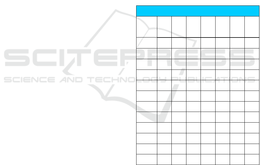
Table 1: Inorganic Chemical Pollution Data for January -

December 2017.

INORGANIC CHEMICAL

MONTH

pH BOD COD DO

Total

Fosfat

NO3-N NH3-N

mg/L mg/L mg/L mg/L mg/L mg/L mg/L

January 7,30 5,70 16,97 6,90 0,322 1,389 0

February 7,60 7,90 26,15 6,40 0,171 2,104 0,110

March 6,80 5,90 20,14 6,90 0,159 0,687 0,048

April 5,80 5,90 15,81 6,80 0,183 1,403 0,095

May 7,50 5,65 13,800 6,60 0,092 0,685 0,017

June 6,40 9,05 28,500 6,00 0,127 0,969 0,102

July 6,20 9,95 21,870 5,20 0,184 1,338 0,098

August 6,40 8,50 29,520 5,20 0,049 3,846 0,113

September 6,3 7,55 24,17 5,8 0,066 0,767 0,162

October 6,5 4,75 17,31 6,8 0,098 0,549 0,108

November 6,1 7,05 20,76 5,9 0,069 1,818 0,029

December 7,1 5,10 15,66 6,7 0,028 1,589 0,067

3.1 pH Value

The pH data used is secondary data obtained from the

BPSDA of Bodowoso Regency in January to

December 2017. Forecasting analysis in modeling

used data from January to September. Table 1 can be

seen that the pH value in the month period ranged

from 5.8 – 7.6. The distribution pattern of the pH data

(Figure 1) in the range of the observation period was

first tested to see if the data was stationary or not.

iCAST-ES 2021 - International Conference on Applied Science and Technology on Engineering Science

104

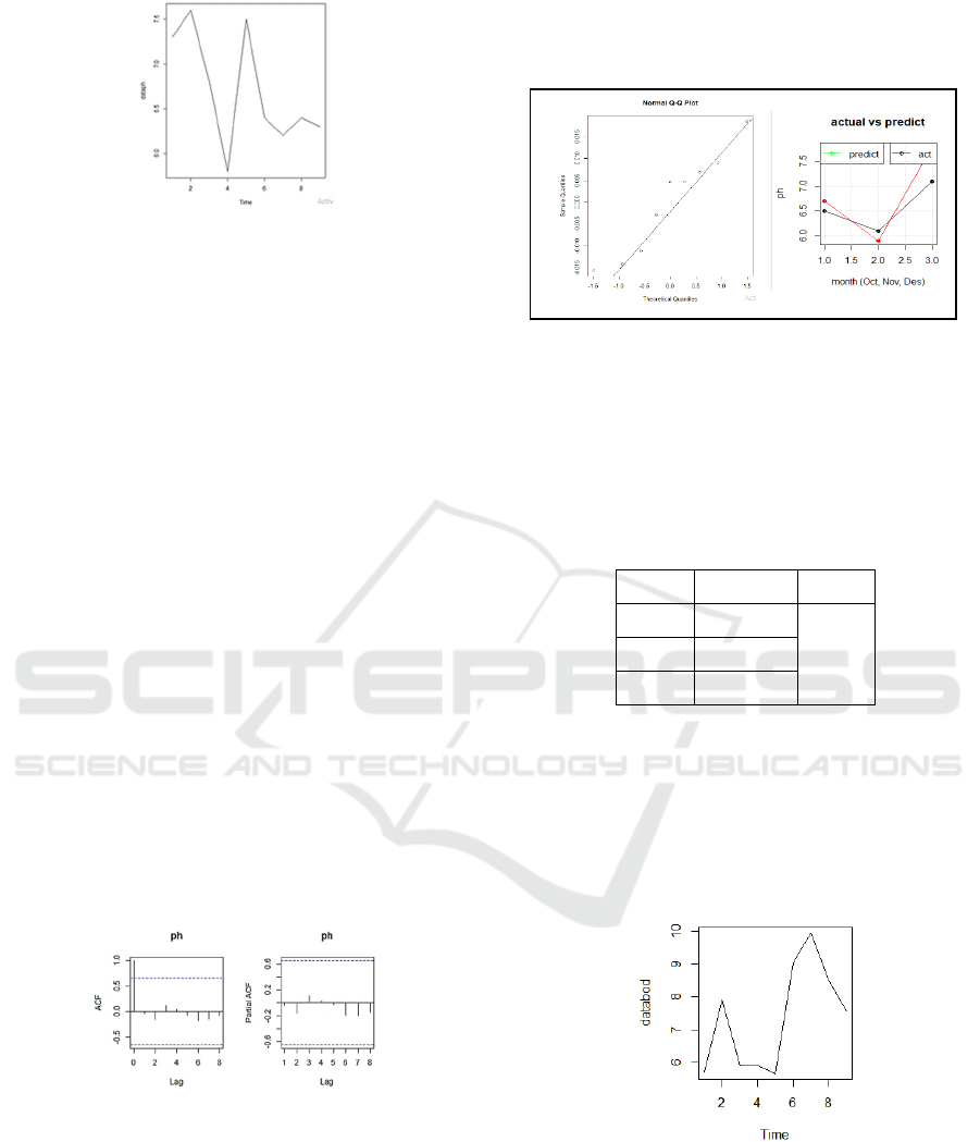
Figure 1: pH Value January-September 2017.

The first step that must be done is to look at the

stationarity of the data, because the condition for

forming a time series analysis model is to assume that

the data is in a stationary state. The time series is said

to be stationary if there is no change in trend, either

in the mean or in the variance. In other words, the

time series is stationary if there is relatively no sharp

increase or decrease in the value of the data. The

stationaryness of the data on the variance can be seen

from the results of the Box-Cox Transformation

where it is said to be stationary if the rounded value

is 1.

The test results by using the powertransform

command found in R -Studio on the data used to get

a value of -1,188 so that it is necessary to transform

so that the value approaches 1. The stationary test of

the data on the variance was carried out using the Box

Cox transformation. After the data is stationary on the

variance, a stationary test is carried out on the

average. The next step for ARIMA modeling is model

identification. The goal is to obtain a provisional

ARIMA model for wind speed data. ACF and PACF

plots are shown in Figure 2. The Dickey-Fuller test

shows that the transformed data has a P-Value of

0.01. This value indicates if the pH value data that has

been transformed does not need to be differencing.

Figure 2: ACF and PACF Plot for pH.

Figure 2 is a plot of ACF and PACF on the parameters

of pH values in January-September. ACF and PACF

plots are used to determine the best ARIMA model in

forecasting future data. The results of the analysis

show that the ARIMA (3,0,0) model is the best with

an AIC value of 51,63. The residual independence

test between lags in the ARIMA (3,0,0) model was

used with the Box-Ljung method and obtained a P-

Value of 0.886. The normality test for the residuals

was carried out using the Shapiro-Wilk method with

the P-value obtained at 0.481.

Figure 3: Normal Q-Q Plot and Forcasting Performance.

The ARIMA (3,0,0) model obtained is used for

forecasting in the next three months. From the test

results, the RMSE value obtained is 0.581. Actual and

predicted pH values in September - December were

obtained at 6.65 and 6.67, 6.1 and 6.72, 7.1 and 6.64.

Table 2: pH Value Actual and Prediction.

Actual Prediction RMSE

6,5 6,67

0,581

6,1 6,72

7,1 6,64

3.2 BOD (Biological Oxygen Demand)

BOD value in the month period ranged from 5,7 – 9,9

mg/L. The distribution pattern of the BOD data

(Figure 4) in the range of the observation period

(January-September) was first tested to see if the data

was stationary or not.

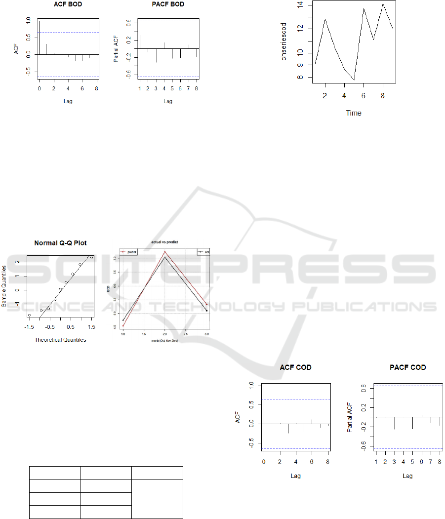
Figure 4: BOD Value January-September 2017.

The test results by using the powertransform

command found in R -Studio on the data used to get

a value of -0.55218 so that it is necessary to transform

so that the value approaches 1. The next step for

ARIMA modeling is model identification. The goal is

to obtain a provisional ARIMA model for wind speed

ARIMA Modeling for Prediction of Inorganic Chemical Pollution in the Kalitambong Watershed, Bondowoso Regency

105

data. ACF and PACF plots are shown in Figure 5. The

Dickey-Fuller test shows that the transformed data

has a P-Value of 0.01.

Figure 5: ACF and PACF Plot for BOD.

Figure 5 is a plot of ACF and PACF on the parameters

of BOD values in January-September. The results of

the analysis show that the ARIMA (2,0,0) model is

the best with an AIC value of 42.7. The residual

independence test between lags in the ARIMA (2,0,0)

model was used with the Box-Ljung method and

obtained a P-Value of 0,481. The normality test for

the residuals was carried out using the Shapiro-Wilk

method with the P-value obtained at 0.762.

Figure 6: Normal Q-Q Plot and Forcasting Performance

BOD.

The ARIMA (2,0,0) model obtained is used for

forecasting in the next three months. From the test

results, the RMSE value obtained is 2.928. Actual and

predicted BOD values in September - December were

obtained at 4.75 and 7.05 and 7.25, 5.1 and 5.33.

Table 3: BOD Value Actual and Prediction.

Actual Prediction RMSE

4,75 4,54

0,581

7,05 7,25

5,1 5,33

3.3 COD (Chemical Oxygen Demand)

COD value in the month period ranged from 13,8 –

29,52 mg/L. The distribution pattern of the COD data

(Figure 7) in the range of the observation period

(January-September) was first tested to see if the data

was stationary or not.

Figure 7: COD Value January-September 2017.

The test results by using the powertransform

command found in R -Studio on the data used to get

a value of 0.781 so that it is necessary to transform so

that the value approaches 1. ACF and PACF plots are

shown in Figure 8. The Dickey-Fuller test shows that

the transformed data has a P-Value of 0.2105. This

value indicates if the COD value data need to be

differencing. After differencing 2 times, a P-value of

0.025 was obtained.

Figure 8 is a plot of ACF and PACF on the

parameters of COD values in January-September.

The results of the analysis show that the ARIMA

(0,2,1) model is the best with an AIC value of 34.7.

The residual independence test between lags in the

ARIMA (0,2,1) model was used with the Box-Ljung

method and obtained a P-Value of 0.187. The

normality test for the residuals was carried out using

the Shapiro-Wilk method with the P-value obtained

at 0.551.

Figure 8: ACF and PACF Plot for COD.

The ARIMA (0,2,1) model obtained is used for

forecasting in the next three months. From the test

results, the RMSE value obtained is 2.918. Actual and

predicted COD values in September - December were

obtained at 17.31 and 17.36, 20.76 and 20.32, 15.66

and 16.37 mg/L.

iCAST-ES 2021 - International Conference on Applied Science and Technology on Engineering Science

106

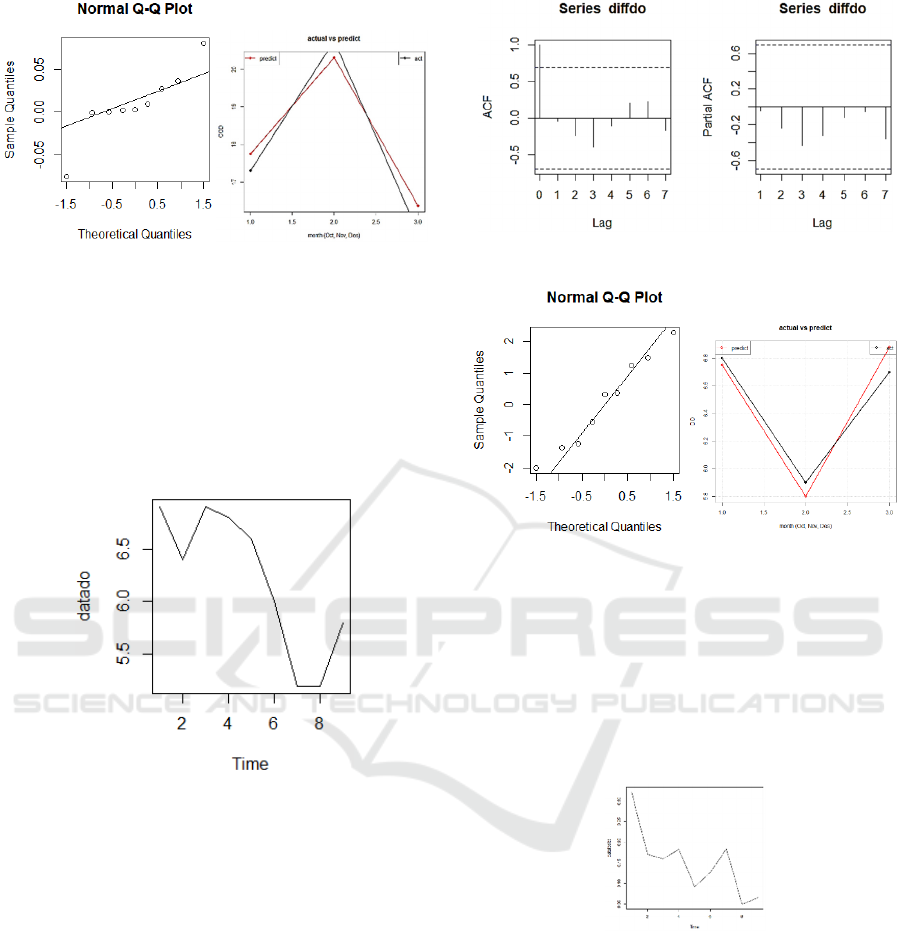
Figure 9: Normal Q-Q Plot and Forcasting Performance

COD.

3.4 DO (Dissolved Oxygen)

DO value in the month period ranged from 5.2-6.9

mg/L. The distribution pattern of the DO data (Figure

10) in the range of the observation period (January-

September) was first tested to see if the data was

stationary or not.

Figure 10: DO Value January-September 2017.

The test results by using the powertransform

command found in R -Studio on the data used to get

a value of 3.979 so that it is necessary to transform so

that the value approaches 1. The next step for ARIMA

modeling is model identification. The goal is to obtain

a provisional ARIMA model for wind speed data.

ACF and PACF plots are shown in Figure 11. The

Dickey-Fuller test shows that the transformed data

has a P-Value of 0.089. After differencing 1 time, a

P-value of 0.019 was obtained.

The ARIMA (0,1,0) model obtained is used for

forecasting in the next three months. From the test

results, the AIC and RMSE value obtained were

13,24 and 0.46. Actual and predicted DO values in

September - December were obtained at 6.8 and 6.75,

5.9 and 5.8, 6.7 and 6.9 mg/L.

Figure 11: ACF and PACF Plot for DO.

Figure 12: Normal Q-Q Plot and Forcasting Performance

DO.

3.5 Total Phosphate

Total Phosphate value in the month period ranged

from 0.092-0.322 mg/L. The distribution pattern of

the total phosphate data (Figure 13) in the range of the

observation period (January-September) was first

tested to see if the data was stationary or not.

Figure 13: Total Phosphate Value January-September 2017.

The test results by using the powertransform

command found in R -Studio on the data used to get

a value of 0.274 so that it is necessary to transform so

that the value approaches 1. The next step for ARIMA

modeling is model identification. The goal is to obtain

a provisional ARIMA model for wind speed data.

ACF and PACF plots are shown in Figure 14. The

Dickey-Fuller test shows that the transformed data

has a P-Value of 0.226. After differencing 1 time, a

P-value of 0.01 was obtained.

ARIMA Modeling for Prediction of Inorganic Chemical Pollution in the Kalitambong Watershed, Bondowoso Regency

107

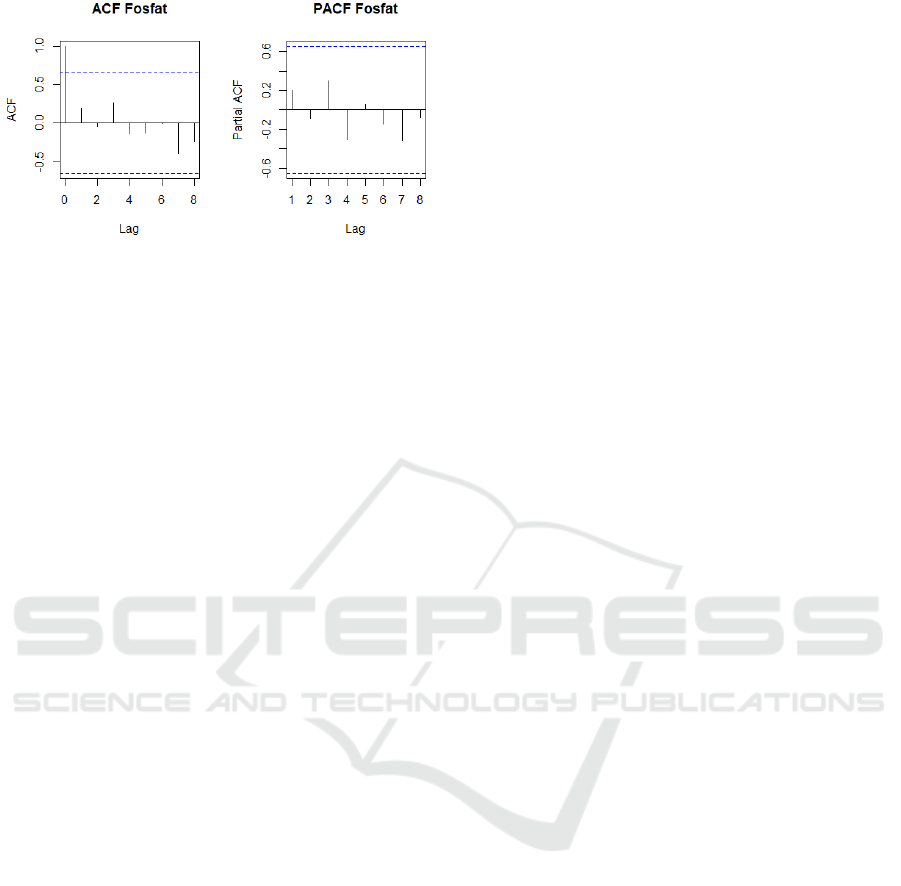
Figure 14: ACF and PACF Plot for Total Phosphate.

The ARIMA (0,1,0) model obtained is used for

forecasting in the next three months. From the test

results, the AIC and RMSE value obtained were 42.7

and 2.92. Actual and predicted total phosphate values

in September - December were obtained at 0.17 and

0.23, 0.16 and 0.26, 0.18 and 0.28 mg/L.

4 CONCLUSIONS

The result of this study is that the best ARIMA model

for ARIMA pH parameter (3,0,0) with AIC value of

51.63 and RMSE 0.581. The best model BOD

parameter is ARIMA (2,0,0) with AIC value of 42.7

and RMSE 2,928. The best model COD parameter is

ARIMA (0,2,1) with AIC of 34.7 and RMSE 2,918.

The DO parameters of the best model are ARIMA

(0,1,0) with AIC and RMSE of 13.24 and 0.46. Total

phosphate parameters with ARIMA model (0,1,0)

with AIC value of 42.7 and RMSE of 2.92.

REFERENCES

Black, P. E. (1996). Watershed hydrology: CRC Press.

Hariono, B., Wijaya, R., Anwar, S., & Wahyono, N. D.

(2018). The Measurement Of Water Quality In

Kalibaru Watershed By Using Storet Method. Paper

presented at the 2018 International Conference on

Applied Science and Technology (iCAST).

Hariono, B., Wijaya, R., Kurnianto, M., Wibowo, M., &

Anwar, S. (2018). Mathematical Model of the Water

Quality in Kalibaru Watershed. Paper presented at the

IOP Conference Series: Earth and Environmental

Science.

Li, L., He, Z., Shields, M. R., Bianchi, T. S., Pain, A., &

Stoffella, P. J. (2018). Partial least squares analysis to

describe the interactions between sediment properties

and water quality in an agricultural watershed. Journal

of Hydrology, 566, 386-395.

Shrestha, N., & Wang, J. (2020). Water Quality

Management of a Cold Climate Region Watershed in

Changing Climate. Journal of Environmental

Informatics, 35(1).

Siami-Namini, S., Tavakoli, N., & Namin, A. S. (2018). A

comparison of ARIMA and LSTM in forecasting time

series. Paper presented at the 2018 17th IEEE

International Conference on Machine Learning and

Applications (ICMLA).

Sugiyarto, S., Hariono, B., Wijaya, R., Destarianto, P., &

Novawan, A. (2018). The impact of land use changes

on carrying capacity of sampean watershed in

Bondowoso Regency. Paper presented at the IOP

Conference Series: Earth and Environmental Science.

Taloor, A. K., Pir, R. A., Adimalla, N., Ali, S., Manhas, D.

S., Roy, S., & Singh, A. K. (2020). Spring water quality

and discharge assessment in the Basantar watershed of

Jammu Himalaya using geographic information system

(GIS) and water quality Index (WQI). Groundwater for

Sustainable Development, 10, 100364.

iCAST-ES 2021 - International Conference on Applied Science and Technology on Engineering Science

108