A Comparative Study of Back-propagation Algorithms:

Levenberg-Marquardt and BFGS for the Formation of Multilayer

Neural Networks for Estimation of Fluoride

R. El Chaal

, M. O. Aboutafail

Engineering Sciences Laboratory. Data Analysis, Mathematical Modeling, and Optimization Team,

Department of Computer Science, Logistics and Mathematics, Ibn Tofail University.

National School of Applied Sciences ENSA, Kenitra 14 000 Morocco

Keywords:

back-propagation algorithm, multilayer perceptron, prediction, optimization, statistical indicators

Abstract: This work describes a comparative approach between the two back-propagation algorithms: the Levenberg-

Marquardt (LM) and the Broyden Fletcher Goldfarb Shanno (BFGS); For the prediction of Fluoride in the

Inaouène basin, using artificial neural networks (ANN) of the multilayer perceptron type (MLP), from the

concentrations of sixteen physicochemical parameters. We have developed several models based on the

evolution of combinations of activation functions and neurons number in the hidden layer. The performance

of the different ANN model training algorithms was evaluated using the mean square error (MSE) and the

correlation coefficient (R). The evaluation shows that the LM training algorithms perform better than the

BFGS training algorithm. The results obtained demonstrate the efficiency of the LM algorithm for the

prediction of Fluoride compared to the BFGS algorithm by MLP type neural networks, as shown by the

statistical indicators ({R = 0.99 and MSE = 0.135 for LM} and {R = 0.95 and MSE = 41.22 for BFGS}).

1 INTRODUCTION

The most popular learning algorithm is Back-

propagation (BP) (Rumelhart et al., 1986), and it is

the most common and widely used supervised

training algorithm for solving approximation

problems, recognition of shapes, classifying and

discovering patterns, and making predictions from

data, and other well-known issues. Based on

statistics, data mining, pattern recognition, and

predictive analyzes. The BP algorithm(BPA) is the

most widely used example of supervised learning

because of the media coverage of some spectacular

applications, such as the demonstration of Sejnowski

and Rosenberg (1987) and Adamson and

Damper(1996), in which BPA is used in a system that

learns to pronounce a text in English(Adamson &

Damper, 1996; Sejnowski & Rosenberg, 1987).

Another success was the prediction of stock market

prices (Refenes & Azema-Barac, 1994) and, the

Comparative study of different artificial neural

network (ANN) training algorithms for atmospheric

https://orcid.org/0000-0002-4705-2006

temperature forecasting in Tabuk, Saudi Arabia

(Perera et al., 2020) and, more recently, a study on

cumulative hazards evaluation for the water

environment(Shi et al., 2021).

The gradient BP technique is a method that

calculates the error gradient for each Neuron in the

network, from the last layer to the first. The

publication history shows that BPA has been

discovered independently by different authors but

under different names. The principle of BP can be

described in three basic steps: routing information

through the network; BP of sensitivities and

calculation of the gradient; and adjust the parameters

by the approximate gradient rule. It is important to

note that BPA suffers from the inherent limitations of

the gradient technique because of the risk of being

trapped in a local minimum. If the gradients or their

derivatives are zero, the network is trapped in a local

minimum. Add to this the slowness of convergence,

especially when dealing with large networks

(Govindaraju, R. S., Rao, 2000) (i.e., for which the

number of connection weights to be determined is

558

El Chaal, R. and Aboutafail, M.

A Comparative Study of Back-propagation Algorithms: Levenberg-Marquardt and BFGS for the Formation of Multilayer Neural Networks for Estimation of Fluoride.

DOI: 10.5220/0010746300003101

In Proceedings of the 2nd International Conference on Big Data, Modelling and Machine Learning (BML 2021), pages 558-565

ISBN: 978-989-758-559-3

essential). To make the optimization more efficient,

we can use second-order methods such as the so-

called Quasi-Newton or modified Newton methods.

2 SECOND-DEGREE

OPTIMIZATION METHOD

(QUASI-NEWTONIAN

METHODS)

2.1 Levenberg-Marquardt

Back-Propagation Method (LM)

The LM algorithm is a variation of Newton's method

(Basterrech et al., 2011), which was designed for

minimizing functions that are sums of squares of non-

linear functions (Bishop, 2006; Dreyfus, 2005). This

is very well suited to artificial neural network (ANN)

training; this is known to be very efficient when

applied to ANN (Ampazis & Perantonis, 2000; Hagan

& Menhaj, 1994), where the root mean square error is

the performance index. Newton's; update for

optimizing a performance index F(x) is

1kkkk

xAg







where

()

AFx



 and

()

gFx





supposing that F(X) is a sum of the square function

(1)

therefore the j th element of the gradient is

(2)

The gradient is written in matrix form

(3)

where(Chen & Zhang, 2012)

(4)

it is the Jacobian matrix. to determine the Hesse

matrix, the element k, j of this matrix would be

(5)

The Hessian matrix can then be expressed in matrix

form

(6)

Where: (7)

If S(x) it is assumed to be minor, the Hessian matrix

can be approximated as

(8)

Substituting (8) and (3) into

kkkk

xAg







, the

Gauss-Newton method is obtained(Scales, 1985)

(9)

From this, the advantage of the Gauss-Newton

method over Newton's standard method is that it does

not require the calculation of second-order

derivatives. A problem with the Gauss-Newton

method is that the matrix

JJ

may not be

invertible. This can be overcome by using the

following modification to the approximate Hessian

matrix:

GH I







To make this matrix invertible, we first assumed that

the eigenvalues and the eigenvectors of H are

respectively the following:





, ,...,





and





, ,...,

zz z

Then

𝑮𝒛







𝑯𝜇𝑰



𝒛



𝑯𝒖



𝜇𝒛



𝜆



𝒛



𝜇𝒛







𝜆



𝜇



𝒛



(10)

herefore, the eigenvectors of G are the same as the

eigenvectors of H, and the eigenvalues of G are

().







can be made positive definite by

increasing



until

()0









for all is,

(11)

(12)

() ()()

Fvv





xxx

()

[()] 2 ()





 





() 2 ()()

FxJxvx

11 1

22 2

() () ()

NN N

vv v

xx x

vv v

xx x

vv v

xx x

 







xx x







() 2 ()() 2()

F xJxJxSx

() () ()







Sx x x

() 2 ()()

FxJxJx

 

kk kk k k

kkk kk

















x x JxJx Jxvx

xJxJx Jxvx

 

kk kkk kk







 





xxJxJx IJxvx

 

kkkkkk





 





xJxJxIJxvx



() () ()

()

() 2 ()

ii i

kj k j kj

vv v

xxxxx







 







 







   







xx x

A Comparative Study of Back-propagation Algorithms: Levenberg-Marquardt and BFGS for the Formation of Multilayer Neural Networks

for Estimation of Fluoride

559

This algorithm has a helpful feature that as



increased, it approaches the steepest descent

algorithm with a small learning rate.

(13)

for large



and if



is decreased to zero, the

algorithm becomes Gauss-Newton.

The algorithm begins with



a set to some small

value (e.g.,

0.01





). If a step does not yield a

smaller value for F(x) then the step is repeated with



multiplied by some factor

1( . . 10)eg







Eventually; F(x) should decrease, as a small step is

taken in the direction of the steepest descent. If the

step does produce a smaller value for F(x) then



divided by



for the next step, so that the algorithm

will approach Gauss-Newton, which should provide

faster convergence.

2.2 Broyden-Fletcher-Goldfarb-Shanno

Back- Propagation Method (BFGS)

Newton's method is based on a quadratic

approximation instead of a linear approximation of

the function F(x). The following approximate

solution is obtained at a point that minimizes the

quadratic function:

(14)

The sequence obtained is

1kkkk

xAg







The main advantage of Newton's method is that it has

a quadratic convergence rate, while the steepest

descent has a much slower, linear convergence rate.

However, each step of Newton's method requires a

large amount of computation. Assuming that the

problem’s dimensionality is N an

()ON

the

floating-point operation is needed to compute the

search direction

. A method that uses an

approximate (Goldfarb, 1970) Hessian matrix in

computing the search direction is the quasi-Newton

method. Let

, be an N*N symmetric matrix that

approximates the Hessian matrix

; Then the

search direction for the quasi-Newton method is

obtained by minimizing the quadratic function:

(15)

it is invertible, a descent direction can be

obtained from the solution of the quadratic program:

(16)

As the matrix,

is to approximate the Hessian of

the function F(x) at



it needs to be updated

from iteration to iteration by incorporating the most

recent gradient information.

The matrix

is updated according to the

following equation(Battiti, 1992; Battiti & Masulli,

1990):

k k kkk k

kk k kk

yy HssH

ys sHs



 

••

(17)

Where

;

kk kk k k

yg g







(18).

2.3 Collection of Data

TAZA is a city located in the northeast of Morocco in

the Taza corridor, a pass where the Rif and Middle

Atlas Mountains meet. Apart from the "corridor"

formed by the valley of the Wadi Inaouen and the

plain of Guercif, the rest of the province is dominated

by mountains. Indeed, the province occupies the area

which connects the Rif to the Middle Atlas, the two

mountain ranges narrowing at the level of the

Touaher pass (559 m above sea level). The Inaouen is

a Moroccan river, that forms near the city of TAZA,

by the confluence of the Boulejraf and Larbaâ wadis,

and borrows from east to west the breach of Taza,

which marks the limit between the Rif and the Middle

Atlas.

Our database consists of 100 surface water

samples (notes) taken in the governorate of Taza (The

Inaouen watershed), between the periods 2014 to

2015, and the collection, transport, and storage of

water samples refer to the protocol and procedures, it

was required by the National Bureau of Drinking

Water. Part of the analysis was carried out on-site

(temperature, dissolved oxygen, etc.). The rest was

done in the Regional University Interface Center

(CURI), backed by the Sidi Mohamed Ben Abdellah

University (USMBA) in Fez.



()

kk kkk





  xx Jxvxx x

   

kkkkkkkkk

FF F



  xxxxgAxxAx

   

kkkkkkkkk

FF F





     xxxxgΔxxHx





d()





  

xx H x

BML 2021 - INTERNATIONAL CONFERENCE ON BIG DATA, MODELLING AND MACHINE LEARNING (BML’21)

560

2.4 Reduction and Preprocessing of

Data

2.4.1 Selection of Inputs

Use The independent (explanatory) variables are the

physical-chemical characteristics determined in these

samples, which are sixteen: Temperature (T ° C), pH,

dissolved oxygen (DO), Conductivity (Cond), total

dissolved solids (TDS) ), Bicarbonate (HCO3), Total

Alkalinity (as CaCO3), Magnesium (Mg), Sodium

(Na), Potassium (K), Chlorides (Cl), Calcium (Ca),

Sulfates (SO4), Nitrate (NO3), Phosphorus (P) and

Ammoniacal nitrogen (NH4),

The dependent variable (to be predicted), it is

Fluoride (F).

The distribution of the database is as follows: 70%

of the samples, chosen at random, from the totality of

the samples, for the learning phase of a predictive

model of the dependent variable. The remaining 30%

samples were used to verify network performance and

to avoid over-learning. This is to test the validity and

performance of the prediction of these models (15%

for the test and 15% for the validation).

2.4.2 Data Formatting

Normalization is a method of preprocessing data that

helps reduce the complexity of models. The input data

(16 independent variables) are raw, untransformed

values. They have very different orders of magnitude.

In order to standardize the measurement scales, these

data are converted into standardized variables.

Indeed, the values of each independent variable (i)

have been normalized with respect to its means and

its standard deviation according to the relation:𝑋𝑣





(Abdallaoui et al., 2015; Bayatzadeh Fard et al., 2017;

Patro et al., 2015)





𝑣











































(19)

With:



𝑣



: Standardized value relating to the variable i.

X𝑣



: Observed value relating to variable i.

𝑋



𝑣



: Average value relating to variable i.

𝑋





𝑣











∑

𝑋



𝑣









(20)

σ𝑣



: standard deviation relating to the variable i.

σ𝑣











∑

𝑋



𝑣



𝑋



𝑣











(21)

The purpose of normalizing the values for all

variables is to avoid very large or minimal

exponential calculations and to limit the increase in

variance with the mean.

The values corresponding to the dependent variables

were also normalized in the interval [0;1] to fit the

requirements of the transfer function used by neural

networks. This normalization was carried out

according to the relation:

𝐘





















(22)

With:



: Standardized value;

Y : Original value;



: Minimum value;



: Maximum value.

2.4.3 Neural Network Implementation with

MATLAB

The multilayer perceptron (MLP) type networks are

much more potent than simple single-layer networks.

The network used in this study consists of three

layers: an input layer, a hidden layer, and an output

layer. The number of neurons in the hidden layer is

not fixed a priori. This is determined during learning.

The neural network simulations were performed

using MATLAB 2018 software.

The implementation of multilayer neural

networks has two parts of the design: determining the

architecture of the network, and an optimization

numerical calculation part. This calculation is the

determination of the synaptic coefficients and the

updating of these coefficients by a supervised

learning algorithm. The algorithm chosen for our

study is the LM and BFGS algorithm. These two

algorithms seek to minimize, by non-linear

optimization methods, a cost function (the mean

squared error (MSE)) which constitutes a measure of

the difference between the actual responses of the

network and its desired responses. This optimization

is done iteratively by modifying the weights as a

function of the gradient of the cost function: the

gradient is estimated by a specific method to neural

networks, called the BP method. It is used by the

algorithm optimization. The weights initialize

randomly before learning.

2.4.4 Evaluation of Performances

For the evaluation of the quality of our predictive

model, and the judgment of these performances,

MATLAB 2018 uses the function of cost, which is

most often used in statistics, and called the least-

squares criterion, and consists of minimizing the sum

of the squares of the residuals, in this case, the

network will learn a discriminant function. The mean

squared error (MSE) is simply given by the sum of

the differences between the target values and the

expected outputs defined for the training set. The

result of the evaluation is expressed in two ways: by





1......16i 

A Comparative Study of Back-propagation Algorithms: Levenberg-Marquardt and BFGS for the Formation of Multilayer Neural Networks

for Estimation of Fluoride

561

statistical indicators and by examining graphs. The

indicators used in this study are the correlation

coefficient (R) and the mean squared error (MSE),

which are defined as follows:

The correlation coefficient:

(23)

The mean squared error (MSE)

(24)

With

obs

is the observed (actual) value of the

studied metal,

predi

is the estimated value of the

metal by the model at observation i,

is the mean

value. The best prediction is when

on the one

hand and SSE, on the other hand, tends towards 1 and

0, respectively.

3 RESULTS AND DISCUSSION

Tests have shown us that to improve the performance

of a model established by MLP (Multilayer

Perceptron) type neural networks, we must modify

the architecture of the network, we change the

number of hidden layers, or the number of hidden

neurons and, or the number of training cycles

(number of iterations). For this, we successively

modified the number of hidden neurons (NHN = 1, 2,

3, ..., 15). In this study, we used two learning

algorithms, called high-performance algorithms LM

and BFGS. For each learning algorithm, we changed

the number of neurons in the hidden layer and the

pairs of transfer functions. Performance was assessed

using the mean square error (MSE) and the

correlation coefficient (R). The algorithms are

implemented and developed in a computer with the

MATLAB 2018 platform. The processor of the

computer is an Intel Core i5-7200U CPU 2.50GHZ

processor, 4 GB RAM.

3.1 Training ANN with LM

Algorithm

Table 1 represents the best performance found for the

different combinations of transfer function pairs for

the LM algorithm; they converge quickly and result in

low values of the mean square error MSE and high

values of the correlation coefficient R in a time of no

more than a few seconds.

Table1: Recap of the best architectures offered by Matlab

for prediction fluoride with algorithm LM.

Hidden

layer

Output

layer

MSE Architecture

Number of

iterations

Tansig Tansig 0,980 33.96 [16-3-1]

Tansig Logsig 0,994 26.14 [16-4-1]

Tansig Purelin 0,910 95.12 [16-5-1]

Logsig Logsig 0,911 92.31 [16-6-1]

Logsig Purelin 0,970 41.4 [16-7-1]

Logsig Purelin 0,999 0.135 [16-8-1]

From this table, we note that:

* The [16-8-1] architecture, with a Logsig function for

the input layer and a Purelin function for the output

layer, gave the best performance for the LM

algorithm: R=0.99 and MSE=0.135.

* The LM algorithm converges with the minimum

number of iterations (22iterations) for all

combinations of transfer functions; this algorithm is

reputed to be very efficient in the approximation of

functions, mainly when the network contains less than

a hundredweight to be updated, which is the case here.

The network reached overtraining after 22 iterations;

it is interesting to keep learning until this stage for the

test to reduce the gradient and improve our network

(Figure.3). From the obtained results in Figure.2; 3,

and 4, we note the different values of training

parameters found in this study:

• Maximum number of iterations (Epochs) = 22

• coefficients of determination = 0.99

• Mean square error (MSE) = 0.135

• Rate of learning (Mu) = 0.0001

• Gradient minimum = 0.875











100

obs obs predi

obs obs p

predi

redi

predi

YY Y













100

MSE

100

obs predi







BML 2021 - INTERNATIONAL CONFERENCE ON BIG DATA, MODELLING AND MACHINE LEARNING (BML’21)

562

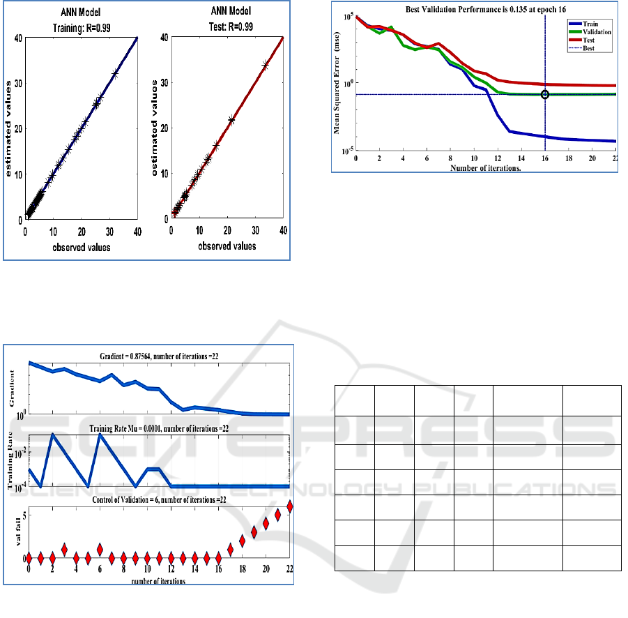
Figure 1: Trend line showing the relationship between the

observed values and values estimated by the MLP model

with algorithm ML for fluoride for the training and test

phase

Figure 2: evolution of the error gradient, the learning rate

and the validation error (for fluoride) as a function of the

number of iterations.

Figure.3 describes network training. It shows that at

the end of the sixteenth iterations, the desired result is

achieved. With eight hidden neurons, the three curves

relating to the evolution of the mean square error of

the three phases converge correctly to the minimum

mean square error (MSE)

Figure 3: the representative graph concerning the

development of the mean square error for a network

architecture [16-8-1].

3.2 Training ANN with BFGS

Algorithm

Table 2 represents the best architecture found for the

different combinations of transfer function pairs for

the BFGS algorithm.

Table 2: Recap of the best architectures offered by Matlab

for prediction Fluoride with algorithm BFGS.

Hidden

layer

Output

layer

MSE Architecture

Number of

iterations

Tansig Tansig 0,920 82.16 [16-3-1]

180

Tansig Logsig 0,916 100.85 [16-4-1]

215

Tansig Purelin 0,901 111.12 [16-5-1]

149

Logsig Logsig 0,953 41.22 [16-6-1]

222

Logsig Purelin 0,932 63.12 [16-7-1]

482

Logsig Purelin 0,945 48.45 [16-8-1]

237

From this table, we note that:

- The [16-6-1] architecture, with a Logsig function for

the input layer and a Purelin function for the output

layer, gave the best performance for the Broyden-

Fletcher-Goldfarb-Shanno algorithm and her indicator

statistical (R=0.95 and MSE=41.22)

The network reached overtraining after 222

iterations; it is interesting to keep learning until this

stage for the test, to minimize the gradient and

improve our network (Figure 6). According to the

results obtained in Figures 5; 6 and 7, we note the

different values of the training parameters found in

this study:

• Maximum number of iterations (Epochs) = 222

• coefficients of determination = 0.95

• Mean square error (MSE) = 41.22

A Comparative Study of Back-propagation Algorithms: Levenberg-Marquardt and BFGS for the Formation of Multilayer Neural Networks

for Estimation of Fluoride

563

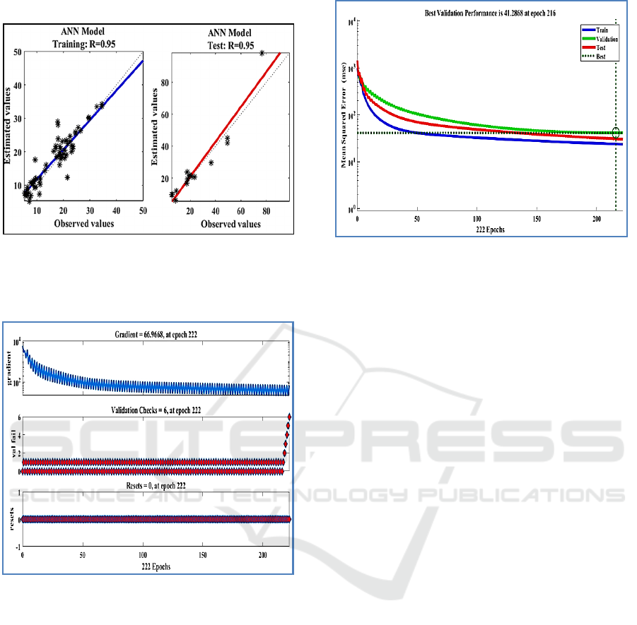
• Gradient minimum = 66.96

Figure 4: Trend line showing the relationship between the

observed values and values estimated by the MLP model

with algorithm BFGS for fluoride for the training and test

phase.

Figure 5: evolution of the error gradient, the learning rate

and the validation error (for fluoride) as a function of the

number of iterations.

Fig.6 describes network training. It shows that at the

end of the 216 iterations, the desired result is achieved.

With six hidden neurons, the three curves relating to

the evolution of the mean square error of the three

phases converge correctly to the minimum mean

square error (MSE=41.28).

Figure 6: the representative graph concerning the

development of the mean square error for a network

architecture [16-6-1].

Figures 3 and 6 give the mean square error (MSE)

values for LM algorithm of ANN. The LM algorithms

showed a lowest MSE value at the point of

convergence. However, the BFGS algorithm took

more epochs (216) to converge to the smallest MSE

(41.22). compared to the LM algorithms training.

Nevertheless, the LM algorithm took only 16 epochs

to reach 0.135 MSE

4 CONCLUSIONS

Artificial neural networks are potent tools for

prediction. They can deal with non-linear problems.

However, they have a significant drawback in the

choice of network architecture, as this choice often

belongs to the user. In our study, we have developed

several models based on the two learning algorithms

LM and BFGS, which are qualified as high-

performing. The results obtained show that the LM

algorithm has the best performance in terms of

statistical indicators (R=0.99 and MSE=0.135) and

convergence speed (22 iterations). Indeed, the model

established by the ML algorithm allows

improvements of up to 4% in the explanation of the

variance compared to that established by the BFGS

algorithm. The evaluation shows that the LM training

algorithms perform better than the BFGS training

algorithm.

Consequently, the analysis results demonstrate

that the LM algorithm has a more efficient approach

than the BFGS for prediction of the Fluoride in

Inaouen basin. However, the BFGS algorithm can be

viewed as a best substitute method.

BML 2021 - INTERNATIONAL CONFERENCE ON BIG DATA, MODELLING AND MACHINE LEARNING (BML’21)

564

In perspective, we can continue in the

development of this subject through the following

suggestions:

 Work on other types of networks such as

recurring networks.

 Use other activation function.

 The results obtained prompt us to reflect

subsequently on the method which makes it

possible to improve the work accomplished

so far. It would be very interesting for

example to use other algorithms.

 Moreover, the models are based on actual

measured data. As a result, they can also be

used to predict future Fluoride

concentrations as a function of

physicochemical parameters.

 Test another RNA architecture to see which

architecture provides a better result.

REFERENCES

Abdallaoui, A., & El Badaoui, H. (2015). Comparative

study of two stochastic models using the

physicochemical characteristics of river sediment to

predict the concentration of toxic metals. Journal of

Materials and Environmental Science, 6(2), 445–454.

Adamson, M. J., & Damper, R. I. (1996). A Recurrent

Network That Learns To Pronounce EnglishText. IEEE

Proceeding of Fourth International Conference on

Spoken Language Processing. ICSLP ’96, 3, 1704–

1707. https://doi.org/10.1109 / ICSLP.1996.607955

Ampazis, N., & Perantonis, S. J. (2000). Levenberg-

Marquardt algorithm with adaptive momentum for the

efficient training of feedforward networks. Proceedings

of the International Joint Conference on Neural

Networks, 1, 126–131.

https://doi.org/10.1109/ijcnn.2000.857825

Basterrech, S., Mohammed, S., Rubino, G., & Soliman, M.

(2011). Levenberg - Marquardt training algorithms for

random neural networks. Computer Journal, 54(1),

125–135. https://doi.org/10.1093/comjnl/bxp101

Battiti, R. (1992). First- and Second-Order Methods for

Learning: Between Steepest Descent and Newton’s

Method. Neural Computation, 4(2), 141–166.

https://doi.org/10.1162/neco.1992.4.2.141

Battiti, R., & Masulli, F. (1990). BFGS Optimization for

Faster and Automated Supervised Learning.

International Neural Network Conference, 757–760.

https://doi.org/10.1007/978-94-009-0643-3_68

Bayatzadeh Fard, Z., Ghadimi, F., & Fattahi, H. (2017). Use

of artificial intelligence techniques to predict

distribution of heavy metals in groundwater of Lakan

lead-zinc mine in Iran. Journal of Mining and

Environment, 8(1), 35–48.

https://doi.org/10.22044/jme.2016.592

Bishop, C. M. (2006). Pattern recognition and machine

learning (Springer (ed.); springer).

Chen, Y., & Zhang, S. (2012). Research on EEG

classification with neural networks based on the

Levenberg-Marquardt algorithm. Communications in

Computer and Information Science, 308 CCIS(PART

2), 195–202. https://doi.org/10.1007/978-3-642-34041-

3_29

Dreyfus, G. (2005). Neural Networks Methodology and

Applications. In Springer Science & Business Media.

Goldfarb, D. (1970). A Family of Variable-Metric Methods

Derived by Variational Means. Mathematics of

Computation, 24(109), 23.

https://doi.org/10.2307/2004873

Govindaraju, R. S., Rao, A. R. (2000). Artificial Neural

Networks in Hydrology. In Water Science and

Technology Library: Vol. 10.1007/97.

https://doi.org/10.1007/978-94-015-9341-0

Hagan, M. T., & Menhaj, M. B. (1994). Training

Feedforward Networks with the Marquardt Algorithm.

IEEE Transactions on Neural Networks, 5

(6), 989–993.

https://doi.org/10.1109/72.329697

Patro, S. G. K., & sahu, K. K. (2015). Normalization: A

Preprocessing Stage. Iarjset, 20–22.

https://doi.org/10.17148/iarjset.2015.2305

Perera, A., Azamathulla, H. M. D., & Rathnayake, U.

(2020). Comparison of different artificial neural

network (ANN) training algorithms to predict the

atmospheric temperature in Tabuk, Saudi Arabia.

Mausam, 71(2).

Refenes, A. N., & Azema-Barac, M. (1994). Neural

network applications in financial asset management.

Neural Computing & Applications, 2(1), 13–39.

https://doi.org/10.1007/BF01423096

Rumelhart, D. E., Hinton, G. E., & Williams, R. J. (1986).

Learning representations by back-propagating errors.

Nature, 323(6088), 533–536.

https://doi.org/10.1038/323533a0

Scales, L. E. (1985). Introduction to Non-Linear

Optimization. In Introduction to Non-Linear

Optimization (springer). Macmillan Education UK.

https://doi.org/10.1007/978-1-349-17741-7

Sejnowski, T. J., & Rosenberg, C. R. (1987). Parallel

systems that learn to pronounce English text. Complex

Systems, 1, 145–168.

Shi, E., Shang, Y., Li, Y., & Zhang, M. (2021). A

cumulative-risk assessment method based on an

artificial neural network model for the water

environment. Environmental Science and Pollution

Research. https://doi.org/10.1007/s11356-021-12540-6

A Comparative Study of Back-propagation Algorithms: Levenberg-Marquardt and BFGS for the Formation of Multilayer Neural Networks

for Estimation of Fluoride

565