Comparative Study of Convolutional Neural Networks-based

Algorithm for Fine-grained Car Recognition

Joseph Sanjaya

, Mewati Ayub

and Hapnes Toba

Faculty of Information Technology, Maranatha Christian University, Jl. Surya Sumantri 65, Bandung, Indonesia

Keywords: Convolutional Neural Networks Model, Object Recognition, Vision Machines.

Abstract: The use of the Deep-Learning model for object recognition in vision machines has been widely applied.

Convolutional Neural Network (CNN) is one of the algorithms which has achieved a significant progress in

object recognition task. An algorithm that has good accuracy and speed is required to recognize a car

specification. This research presents a comparative study of several CNN models for car recognition. This

study is a continuation of previous study about data augmentation in car image recognition using ResNet

architecture. In this study, the CNN architectures which are used in comparison, are ResNet, SqueezeNet, and

EfficientNet. The aim of this study is to find an architecture with optimal performance in car recognition. The

dataset used is a Cars Dataset provided by Stanford University. The methods consist of data pre-processing,

model training and hyper parameter tuning, inferences and comparison. The metrics which were used during

the experiments are accuracy, model size, and speed. Training of each model was performed using computer

with the same specification. The experimental results indicate that EfficientNet model gives the best result

among other models in the context of accuracy, model size, and speed.

1 INTRODUCTION

The development of technology nowadays runs so

fast, many vision machines have supported human

life. Convolutional Neural Networks (CNNs) is an

algorithm that has achieved significant progress for

vision machine's tasks, which are image

classification, objective detection, and semantic

segmentation. CNN algorithm has a strong ability in

feature extraction for an image. The algorithm is often

used in object recognition task, including car model

recognition.

Using vision machines, smart transportation can be

implemented in daily life. An intelligent

transportation system is an implementation of IoT

(Internet of Things) which is integrated with

information technology and an automatic control

system. This system can be implemented in the road

traffic management system to control the traffic in

real-time more accurately (Ke, Shi, Guo, & Chen,

2019). An electronic police system is an

implementation of smart transportation, which uses

https://orcid.org/0000-0002-0574-9147

https://orcid.org/0000-0003-2584-4317

https://orcid.org/0000-0003-0586-8880

technology to identify vehicle license plates. The

identification of license plate can be used to recognize

vehicle that violates traffic rules.

In recognizing vehicles more accurately, the

license plate identification is not enough, it should be

equipped with a vehicle recognition system (Ke &

Y.Zhang, Fine-grained vehicle type detection and

recognition based on dense attention network, 2020).

CNN model is required in object detection with good

accuracy and fast speed. The model should still work

in traffic disorderly conditions. Based on the

requirements, in this study, some object recognition

using CNN algorithms will be explored and evaluated

according to the accuracy, speed, and model size of

each algorithm.

This research is a continuation of a previous study

about data augmentation in car image recognition

using ResNet architecture (Sanjaya & Ayub, 2020).

The aim of this study is to obtain a method to

implement CNN architectures in car recognition, and

to compare the architectures based on accuracy,

speed, and model size metrics. The CNN

Sanjaya, J., Ayub, M. and Toba, H.

Comparative Study of Convolutional Neural Networks-based Algorithm for Fine-grained Car Recognition.

DOI: 10.5220/0010743800003113

In Proceedings of the 1st International Conference on Emerging Issues in Technology, Engineering and Science (ICE-TES 2021), pages 18-25

ISBN: 978-989-758-601-9

architectures used in the comparison, are ResNet,

SqueezeNet, and EfficientNet.

The CNN architectures are chosen regarding the

advantages of each architecture in object recognition.

ResNet architecture has good stability and accuracy

(Zhang & Schaeffer, 2020), SqueezeNet architecture

has a small model size, so the architecture is suitable

for use with IoT (Lee, Ullah, Wan, Gao, & Fang,

2019). EfficientNet architecture has good accuracy

and speed with efficient processing power (Tan & Le,

2019).

The dataset used is the same dataset used in a

previous study (Sanjaya & Ayub, 2020), which is a

Cars Dataset provided by Stanford University, which

contains 16,185 images of 196 car classes

. The

composition of training data and test data is fifty-fifty.

The result of this study is a CNN deep learning model

for each architecture, that can classify a car model and

performance analysis of each model.

The initial hypothesis of each architecture in object

recognition will be explained as follows. CNN model

of ResNet 152 architecture has a deep layer, so it

should recognize complex features properly (He,

Zhang, Ren, & Sun, 2016). It can be assumed that a

model based on this architecture would have better

accuracy. Regarding the deep layer, this model would

have less good speed and model size.

CNN model of SqueezeNet architecture has a wide

layer so it should recognize more features with not

deep layers (Lee, Ullah, Wan, Gao, & Fang, 2019). It

can be assumed that a model based on this

architecture would have a good model size and speed

training with trade-off accuracy.

CNN model of EfficientNet architecture is

obtained from neural network searching against

efficiency and accuracy (Tan & Le, 2019). It can be

assumed that a model based on this architecture

would have good and efficient performance.

2 METHODS

2.1 Research Design

The study uses data augmentation in the previous

study (Sanjaya & Ayub, 2020) to analyze the three

architectures. Performance of CNN model of three

architectures would be measured based on model size,

speed, and accuracy metrics. Figure 1 shows the

stages of the methodology. The flow of the processes

is input data, data preprocessing, training model,

hyper parameter tuning, inferences and comparison.

Data input to this study is car images from

Stanford Cars Dataset (Krause, Stark, Deng, & Fei-

Fei, 2013). Data preprocessing is required to

transform raw image data into prepared data. Data

preprocessing is performed using data augmentation,

that are random crop, rotate, and mixup (Sanjaya &

Ayub, 2020).

CNN model based on ResNet, SqueezeNet, dan

EfficientNet architectures is used as a feature

extraction process. The model will be optimized

using hyper parameter tuning, which focused on the

optimal learning rate parameter. Statistical analysis

will be used in comparative analysis to determine the

optimal model based on accuracy, speed, and model

size metrics.

Accuracy metric in classification is measured

based on formula (1) (Han, Kamber, & Pei, 2012):

accuracy = (TP + TN)/(P+N) (1

)

Where: TP is the number of true positives; TN is the

number of true negatives; P is the number of positives

tuples, and N is the number of negative tuples.

Speed metric is required to compare time

efficiency and computation power for each CNN

model (Ning, Guan, & Shen, 2019) . Speed metric is

measured from the time needed for executions in

minutes.

Model size metric in deep learning can be

measured based on the width and the depth of neural

network. The metric is important, when model size

increases caused of the expansion of input size.

Adjustment of image data and model in memory

between CPU and GPU causes the training time to

increase. There is a trade-off between speed and

model size (Deng, Li, Han, Shi, & Xie, 2020).

2.2 Hardware Specification

In order to give balanced results, hardware

specification used in model training and execution

should have the same strength, mainly GPU, CPU,

and RAM. Table 1 shows the hardware specification.

2.3 Model Training

In order to give balanced results, hardware

specification used in model training and execution

should have the same strength, mainly GPU, CPU,

and RAM.

Hyper-parameter tuning will be explored in the

beginning of experiments. Deep learning parameters

which tuned are learning rate and batch size (Smith,

2018). In contrast to learning rate, batch size will

affect time of training model, because batch size is

limited by hardware memory.

Comparative Study of Convolutional Neural Networks-based Algorithm for Fine-grained Car Recognition

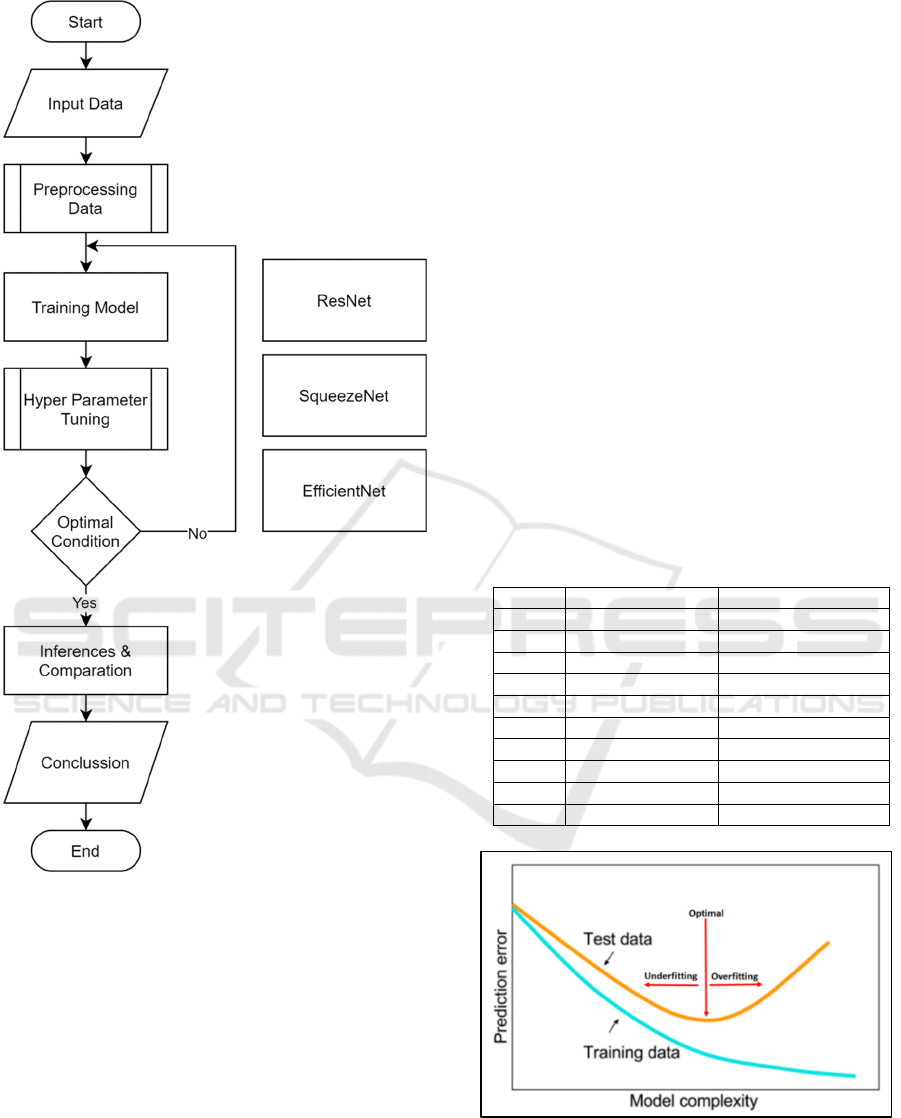
Figure 1: Research Design

Smith recommended to using the largest batch size

that could be accommodated by hardware memory.

The recommendation allows to utilize larger learning

rate (Smith, 2018). When training is executed on a

server with several GPUs, batch size total is

calculated as batch size on each GPU multiplied by

the number of GPU.

Based on the batch size, experiments are performed

from the largest one until the smallest one, until Out-

of-Memory (OOM) error is not occurred. The

experiments are executed from batch size 248 and

decreased by 24 per step up to no OOM error. The

results on ResNet 152 model can be seen on Table 2.

From the Table 2, the hardware specification on

Table 1 is only able to run the training with batch size

32. This is caused by image resolution size (300px to

1500px) and ResNet 152 architecture, which require

large memory size.

Underfitting is a condition when machine learning

model cannot decrease error, both in training and

testing phase. On the other side, overfitting is a

condition when machine learning model is too strong,

so generalization error increases (Smith, 2018).

Figure 2 shows trade-off between underfitting and

overfitting. If learning rate (LR) is too small, then

overfitting will be happened. Large learning rate will

support training regularization, but if learning rate is

too large, training will be cluttered.

The results of batch size hyper parameter tuning of

SqueezeNet and EfficientNet model can be seen on

Table 3. On the Table 3, the hardware specification

on Table 1 is only able to run the training with batch

size 56. ResNet 152 model are different from

SqueezeNet model, which has a wide CNN

architecture, so SqueezeNet can capture features with

smaller memory. EfficientNet model has the same

batch size as SqueezeNet.

Table 1: Batch size hyper-parameter tuning of ResNet 152.

# Batch size Status

1 248 OOM

2 224 OOM

3 200 OOM

4 176 OOM

5 152 OOM

6 128 OOM

7 104 OOM

8 80 OOM

9 56 OOM

10 32 Success

Figure 2: Model Complexity (Smith, 2018).

ICE-TES 2021 - International Conference on Emerging Issues in Technology, Engineering, and Science

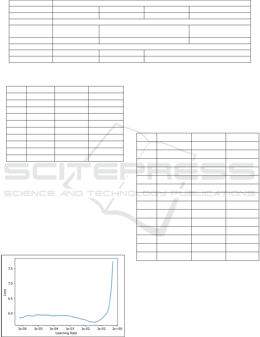
Table 2: Hardware specification.

Name of GPU GTX 1080 Max - Q

Memor

e Memor

asit

GPU Cloc

Memor

Cloc

Boost Cloc

GDDR5X 8192MB 1297 MHz 1251 MHz 1436 MHz

Name of CPU Intel Core i7 7700HQ

Lithography

technolo

Clock Speed Cores Threads

14 nm 2.80 GHz 4 8

Name of RAM SAMSUNG 19FAC364

Type Channel Memory Capasity Maximum Bandwidth

DDR4 Dual 16 GB 1200 MHz

Table 3: Batch size hyper-parameter tuning of SqueezeNet

and EfficientNet.

#Exp. Batch size SqueezeNet EfficientNet

1 248 OOM OOM

2 224 OOM

OOM

3 200 OOM

OOM

4 176 OOM

OOM

5 152 OOM

OOM

6 128 OOM

OOM

7 104 OOM

OOM

8 80 OOM

OOM

9 56 Success

Success

10 32 Success Success

3 RESULTS AND DISCUSSION

At each batch, neural network would be trained with

increased learning rate exponentially. Training batch

was divided into two different experiments in order to

obtain an optimal learning rate interval (Smith, 2017).

Hyper parameter tuning experiment of learning

rate on ResNet 152 model is executed using fast.ai

package (function lr_find()). Figure 3 shows

visualization between loss and learning rate from the

first experiment.

Figure 3: Learning rate of ResNet 152 model (first

experiment).

In Figure 3, an optimal learning rate interval

happened when the loss function declined quickly, so

the best learning rate resulted from the first

experiment is an area that has small loss, that is, from

1e-02 to 1e-01. The result of training using those

learning rates can be seen on Table 4.

Table 4: Experiment of training LR range for Resnet 152-

Epoch Train Loss Valid Loss Accuracy

1 4.325618 3.377519 0.240172

2 3.174334 3.768307 0.180590

3 3.214476 3.275414 0.264128

4 2.790483 2.558635 0.358722

5 2.484006 2.819357 0.330467

6 2.116244 2.070632 0.455774

7 1.857780 1.635659 0.567568

8 1.557437 1.435014 0.610565

9 1.276098 1.072250 0.700246

10 1.024269 0.921169 0.748157

11 0.793735 0.812245 0.773956

12 0.634392 0.745959 0.787469

13 0.519093 0.704684 0.800983

14 0.503253 0.703171 0.802211

In Table 4, model training is performed until epoch

14, because the result after epoch 14 trends to

convergent. The training resulted good accuracy

performance.

Comparative Study of Convolutional Neural Networks-based Algorithm for Fine-grained Car Recognition

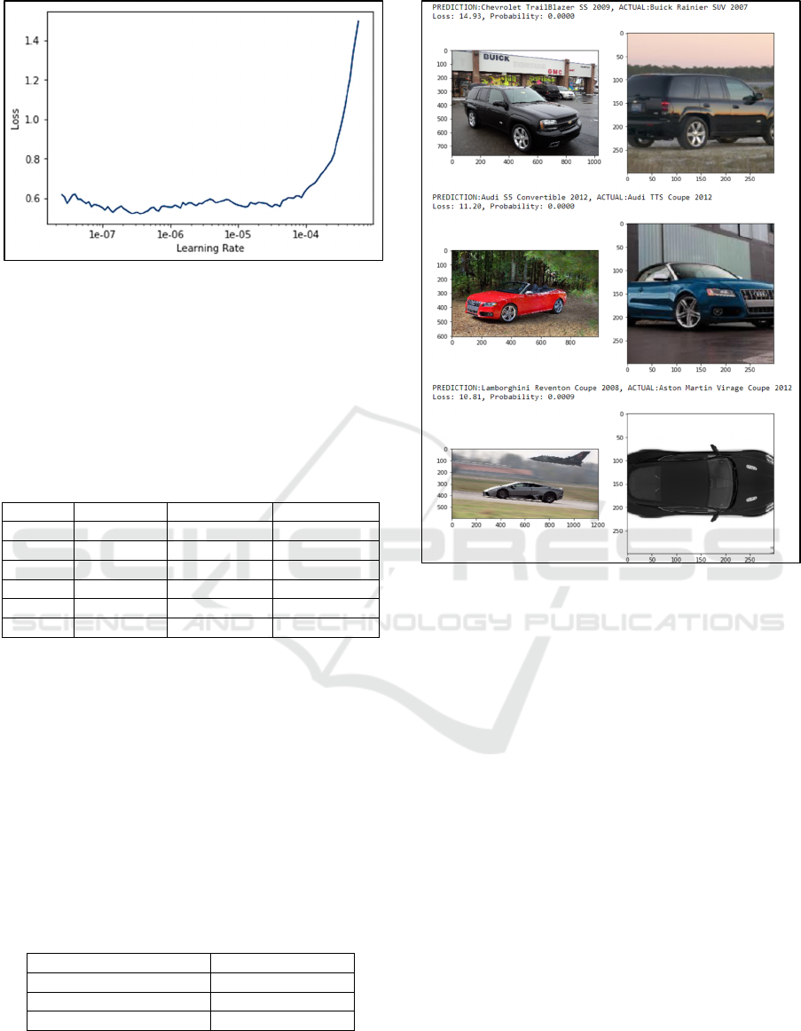
Figure 4: Learning rate of ResNet 152 model (second

experiment).

Figure 4 shows results from second experiment

training of ResNet 152, with LR from 1e-7 to 1e-6.

The result of training using those learning rate can be

seen on Table 5, which shows better accuracy

(82.55%).

Table 5: Experiment of training LR range for Resnet 152-

och Train Loss Valid Loss Accurac

1 0.966993 1.169178 0.699017

2 1.463537 1.227771 0.680590

3 1.152164 0.982462 0.732187

4 0.871343 0.710956 0.798526

5 0.589137 0.630260 0.818796

6 0.456042 0.602334 0.825553

Model evaluation was conducted using Test Time

Augmentation (TTA). TTA performed data

augmentation as neural transfer style, flipping

images, cropping to test dataset. After the model

predicted class label of augmented test data, scores

were collected to calculate final prediction of origin

images (Nalepa, Myller, & Kawulok, 2020). The

results can be seen in Table 6.

For further observations, experiments were

conducted on images which are top losses and most

confused to the model. Classification results of top

losses on ResNet 152 model can be seen in Figure 5.

Table 6: Model evaluation of ResNet 152.

Metrics Value

ccurac

(

)

82.95

odel size (MB) 208.06

Speed (Minutes) 24:45

Figure 5: Classification result of ResNet 152 top losses

data.

Figure 6 shows classification results of most

confused of Resnet 152 model. In Figure 7, the best

learning rate resulted from the first experiment of

SquuezeNet model is an area that has small loss, that

is from 1e-02 to 1e-01. The result of training using

those learning rate can be seen on Table 7.

In Table 7, model training is performed until epoch

14, because the result after epoch 14 trends to

convergent. The training resulted bad accuracy

performance. The second experiment was executed to

get better accuracy. Figure 8 shows the best learning

rate resulted from the second experiment, which is an

area that has small loss, that is from 1e-06 to 1e-05.

The results of second experiment training can be seen

on Table 8, which shows better accuracy (57.24%).

ICE-TES 2021 - International Conference on Emerging Issues in Technology, Engineering, and Science

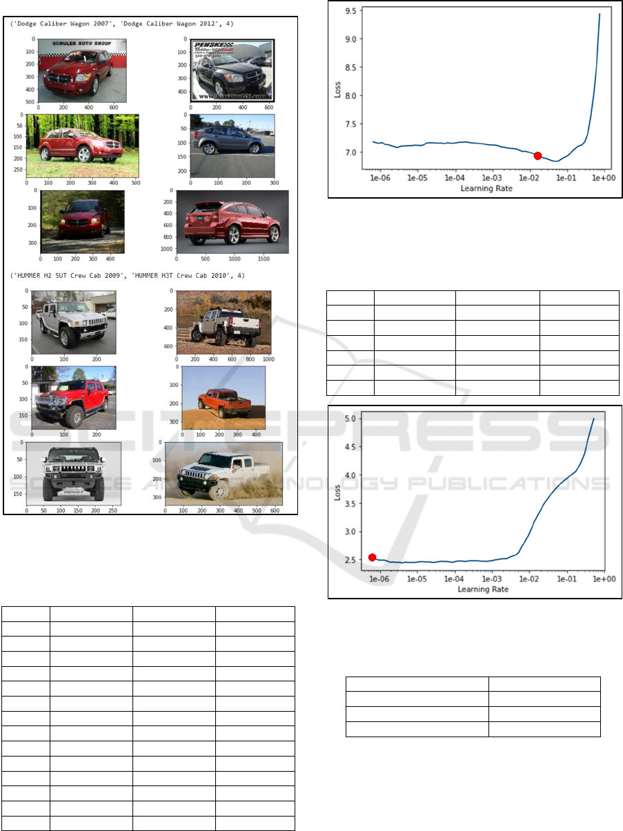
Figure 6. Classification result of ResNet 152 most confused

data.

Table 7: Experiment of training LR range for SqueezeNet-

Epoch Train Loss Valid Loss Accurac

1 6.163468 4.424913 0.100737

2 4.999869 3.619730 0.191646

3 4.526335 3.339163 0.245086

4 4.119049 2.996984 0.306511

5 3.798199 2.778760 0.343980

6 3.601222 2.588148 0.378378

7 3.468006 2.527634 0.398034

8 3.342122 2.387317 0.426290

9 3.169286 2.298042 0.438575

10 3.010396 2.204117 0.472973

11 2.875496 2.100137 0.496314

12 2.724763 2.057748 0.507985

13 2.689825 2.023018 0.516585

14 2.626248 2.030500 0.511671

Figure 7: Learning rate of SqueezeNet model (first

experiment).

Table 8: Experiment of training LR range for SqueezeNet –

Epoch Train Loss Valid Loss Accurac

1 2.595495 1.943847 0.533784

2 2.469271 1.789647 0.562654

3 2.466382 1.779467 0.565725

4 2.489725 1.771083 0.567568

5 2.470081 1.776281 0.565111

6 2.469402 1.777249 0.572482

Figure 8: Learning rate of SqueezeNet model (second

experiment).

Table 9: Model evaluation of SqueezeNet.

Metrics Value

Accurac

(

)

57.22

Model size

(

)

10.06

Speed (minutes) 14:11

Table 9 shows model evaluation result of SqueezeNet.

In Figure 9, the best learning rate resulted from the

first experiment of EfficientNet model is an area that

has small loss, that is from 1e-03 to 1e-02. The result

of training using those learning rate can be seen on

Table 10.

Comparative Study of Convolutional Neural Networks-based Algorithm for Fine-grained Car Recognition

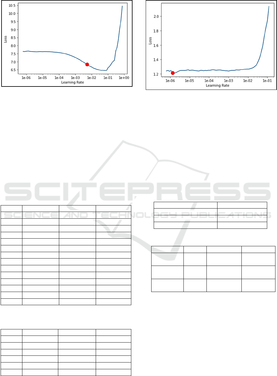
Figure 9: Learning rate of EfficientNet model (first

experiment).

In Table 10, model training is performed until

epoch 14, because the result after epoch 14 trends to

convergent. The training resulted good accuracy

performance. The second experiment was executed to

get better accuracy.

Figure 10 shows the best learning rate resulted

from the second experiment, which is an area that has

small loss, that is from 1e-06 to 1e-05. The results of

second experiment training can be seen on Table 11,

which shows better accuracy (88.57%).

Table 10: Experiment of training LR range for EfficientNet-

och Train Loss Valid Loss Accurac

1 3.895927 2.443662 0.378378

2 3.164658 2.917843 0.336609

3 3.153092 3.931816 0.228501

4 3.112244 2.622782 0.362408

5 2.836884 2.377069 0.420147

6 2.558743 1.697689 0.560197

7 2.310468 1.386264 0.641892

8 2.102232 1.067460 0.730344

9 1.867059 0.899833 0.758600

10 1.693708 0.692391 0.818796

11 1.510015 0.599369 0.856265

12 1.378668 0.540748 0.872850

13 1.327494 0.506629 0.883907

14 1.297732 0.505953 0.885749

Table 11: Experiment of training LR range for EfficientNet-

och Train Loss Valid Loss Accurac

1 1.282915 0.509046 0.883907

2 1.274822 0.513583 0.884521

3 1.279225 0.506601 0.885135

4 1.275859 0.510035 0.884521

5 1.283290 0.505331 0.885749

6 1.270210 0.509779 0.884521

Figure 10: Learning rate of EfficientNet model (second

experiment).

Table 12 shows model evaluation result of EfficientNet.

Table 13 shows the results of all experiments of three

model. Table 13 indicates that SqueezeNet has the

best result for two metrics, that are model size and

speed. Architecture SqueezeNet is very suitable to be

applied in real time application, which accuracy is not

important. As an example, SqueezeNet can be

implemented in IoT (Internet of Things) applications,

which have a limited memory and processing power

in classification tasks.

Table 12: Model evaluation of EfficientNet.

Metrics Value

Accuracy (%) 84.88

Model size

(

)

107.201

eed

(

minutes

)

23:55

Table 13: Results summary of experiments of each model.

Metrics ResNet SqueezeNet EfficientNet

Accuracy

(

)

82.95 57.22 84.88

Model Size

(

)

208.06 10.06 107.201

Speed

(Minutes)

24:45 14:11 23:55

EfficientNet has better accuracy, model size, and

speed compared to ResNet as shown in Table 13. The

best performance is achieved by EfficientNet, this

model is very suitable for classification tasks, which

required high accuracy.

4 CONCLUSIONS

Implementation of three CNN models for car

recognition task has been performed and evaluated

using TTA. The experiment result shows that

ICE-TES 2021 - International Conference on Emerging Issues in Technology, Engineering, and Science

accuracy of Resnet 152 model is 82.97%. The worst

accuracy (57.22%) is obtained by SqueezeNet model

and the best accuracy (84.88%) is achieved by

EfficientNet model. CNN model of EfficientNet

architecture achieved the optimal results, which can

be seen from the accuracy, model size, and speed

metrics. SqueezeNet obtained the best model size and

speed, so SqueezeNet is suitable for real time

implementation with trade-off accuracy. Further

research is needed to explore the optimization of

SqueezeNet to obtain better performance.

REFERENCES

Deng, B. L., Li, G., Han, S., Shi, L., & Xie, Y. (2020).

Model Compression and Hardware Acceleration for

Neural Networks: A Comprehensive Survey.

Proceedings of IEEE, 108(4), 485-532.

Han, J., Kamber, M., & Pei, J. (2012). Data Mining

Concepts and Techniques. Waltham: Elsevier, Inc.

He, K., Zhang, X., Ren, S., & Sun, J. (2016). Deep Residual

Learning for Image Recognition. IEEE Conference on

Computer Vision and Pattern Recognition (CVPR) (pp.

770-778). Las Vegas: IEEE.

Ke, X., & Y.Zhang. (2020). Fine-grained vehicle type

detection and recognition based on dense attention

network. Neurocomputing, 399, 247-257.

Ke, X., Shi, L., Guo, W., & Chen, D. (2019). Multi-

Dimensional Traffic Congestion Detection Based on

Fusion of Visual Features and Convolutional Neural

Network. IEEE Transactions on Intelligent

Transportation Systems,, 20(6), 2157-2170.

Krause, J., Stark, M., Deng, J., & Fei-Fei, L. (2013). 3D

Object Representations for Fine-Grained

Categorization. IEEE International Conference on

Computer Vision Workshops (ICCVW) (pp. 554-561).

Sydney: IEEE.

Lee, H., Ullah, I., Wan, W., Gao, Y., & Fang, Z. (2019).

Real-Time Vehicle Make and Model Recognition with

the Residual SqueezeNet Architecture. Sensor, 19(5),

982.

Nalepa, J., Myller, M., & Kawulok, M. (2020). Training-

and Test-Time Data Augmentation for Hyperspectral

Image Segmentation. IEEE Geoscience and Remote

Sensing Letters, 17(2), 292-296.

Ning, L., Guan, H., & Shen, X. (2019). Adaptive Deep

Reuse: Accelerating CNN Training on the Fly. IEEE

35th International Conference on Data Engineering

(ICDE), (pp. 1538-1549). Macao.

Sanjaya, J., & Ayub, M. (2020). Augmentasi Data

Pengenalan Citra Mobil Menggunakan Pendekatan

Random Crop, Rotate, dan Mixup. Jurnal Teknik

Informatika dan Sistem Informasi, 6(2), 311-323.

Smith, L. N. (2017). Cyclical Learning Rates for Training

Neural Networks. IEEE Winter Conference on

Applications of Computer Vision (WACV) (pp. 464–

472). Santa Rosa: IEEE.

Smith, L. N. (2018). A disciplined approach to neural

network hyper-parameters: Part 1 -- learning rate,

batch size, momentum, and weight decay. Retrieved

from https://arxiv.org/abs/1803.09820

Tan, M., & Le, Q. V. (2019). EfficientNet: Rethinking

Model Scaling for Convolutional Neural Networks.

Proceedings of the 36th International Conference on

Machine Learning (ICML), (pp. 6105-6114). Long

Beach.

Zhang, L., & Schaeffer, H. (2020). Forward Stability of

ResNet and Its Variants. Journal of Mathematical

Imaging and Vision, 62(3), 328-351.

Comparative Study of Convolutional Neural Networks-based Algorithm for Fine-grained Car Recognition