
Comparison of Machine Learning Techniques to Forecast the Output
Power of Photovoltaic Panels using Multiple Prediction Factors
Souhaila
Chahboun
a
, Mohamed Maaroufi
Mohammadia School of Engineers, Mohammed V University in Rabat, Morocco
Keywords: Solar energy, Photovoltaic output power, Prediction, Regression analysis, Machine learning.
Abstract: When the energy transition is unavoidable and artificial intelligence is omnipresent, renewable energies
production prediction is becoming a popular concept, especially with the availability of big data sets and the
crucial need to forecast these energies known to have a random nature. Thus, the critical goal of this paper is
to compare the performance of two approaches, including traditional linear regression and non-linear
regression analysis, for the forecasting of the power trends of photovoltaic panels, and thus determine the
model giving the most reliable predictions. This study revealed that the non-linear approach provides the best
prediction result since it achieved an R²=94% in the testing phase, and its root mean square error is the lowest
value RMSE=0.51 Kw.
1 INTRODUCTION
1.1 State of the Art
The prediction of the photovoltaic (PV) power is an
important factor for the correct decision-making in
terms of funding and operations scheduling,
economic dispatch of solar energy (Moslehi et al.,
2018) and maintenance operations (Kaaya et al.,
2020). However, PV power is often brutal to predict
since various factors impact its value, including the
local environment, technological advancements, and
installation characteristics. (Jordan et al., 2017).
Therefore, to meet all these challenges and needs,
several advanced methods have been suggested by
researchers.
On one side, the application of physical models is
a decisive and critical element in forecasting the PV
power. In these models, mathematical equations
incorporate the relationship and interaction between
physical parameters, solar irradiation models and
other components of the atmosphere (Sobri et al.,
2018). This approach encounters several constraints
due to the continuous need for technical datasheets of
PV systems (Maitanova et al., 2020), uncertainties
that can come from environmental data and
simplifications considered in models, which strongly
affects the accuracy of forecasts.
a
https://orcid.org/0000-0001-6011-8164
On the other side, data-driven approaches use
historical data to recognize the relationship between
the explanatory (predictor) and explained (outcome)
parameters. Complex systems employ these models,
where the elaboration of physical models could be
more complicated and expensive (Theocharides et al.,
2018)(Wang et al., 2017). They include statistical
methods and machine learning techniques.
For applications in the PV field, authors have
conducted several surveys and elaborated different
predictive models based on data interpretation and
review to estimate the PV-produced power. For
instance, Antonanzas et al. (Antonanzas et al., 2016)
provided a comprehensive overview of the most up-
to-date techniques for PV power predictions such as
k-nearest neighbour, random forest, and support
vector regression. Ramli et al. (Ramli et al., 2019)
used the k-nearest neighbour method and compared it
to artificial neural networks. Golder et al. (Golder et
al., 2019) explored three Data mining approaches for
PV power prediction, including multi-layer
perceptrons, support vector machines and long short-
term memory. Kayri et al. (Kayri et al., 2017)
employed random forest and artificial neural
networks for PV power forecast.
In this article, we
investigated the performance of two machine learning
methods for the hourly forecasting of the PV power.
We evaluated the efficacy of the examined methods
474
Chahboun, S. and Maaroufi, M.
Comparison of Machine Learning Techniques to Forecast the Output Power of Photovoltaic Panels using Multiple Prediction Factors.
DOI: 10.5220/0010736800003101
In Proceedings of the 2nd International Conference on Big Data, Modelling and Machine Learning (BML 2021), pages 474-478
ISBN: 978-989-758-559-3
Copyright
c
2022 by SCITEPRESS – Science and Technology Publications, Lda. All rights reserved

using the most widely used performance metrics.
Finally, we used residual analysis to visually test the
predictive models. The rest of this work is structured
as follows. Section 2 introduces the methods used in
the study. Section 3 provides results analysis and,
Section 4 provides the conclusion of this paper.
1.2 Position of the Problem
PV power forecasting is considered a difficult task
due to the variability of meteorological conditions.
Thus, the contribution of this work is to take
advantage of the development of machine learning
techniques to predict the power of solar PV panels as
one of the keys to its integration in a diversified
electrical network.
In literature, several surveys exist on solar power
predictions using machine learning approaches.
However, the literature still lacks a comprehensive
review of their performance. Most current studies
employ datasets dependent on a specific time of the
year, making it difficult to evaluate the final results.
Moreover, only a few examinations have compared
linear and non-linear models to identify the approach
offering the best accuracy.
This paper examined the use of multiple linear
regression and multivariate adaptive regression
splines, not widely employed in the field of solar
energy forecast using the same set of data.
2 MATERIALS AND METHODS
2.1 Data Source and Description
For the PV power prediction, we present the input
data as follows:
2.1.1 Meteorological Data
We retrieved the meteorological inputs from the
dataset modern age hindsight web service, which are:
Relative Humidity (RH) %, Wind speed (WS) m/s,
Wind direction (WD) deg, Short-wave irradiation
(Irr) wh/m², Ambient Temperature (Tamb) °C and
Pressure (P) hPa.
2.1.2 Solar Radiation Data
We collected the irradiation inputs from the
Copernicus Atmosphere Monitoring Service (CAMS)
(Gschwind et al., 2019). These inputs are Top of
Atmosphere irradiation (TOA), Clear sky global
irradiation on the horizontal plane (CSGHI), Clear
sky beam irradiation on the horizontal plane
(CSBHI), Clear sky diffuse irradiation on the
horizontal plane (CSDHI), Clear sky beam irradiation
on the mobile plane (CSBNI), Global irradiation on
the horizontal plane (GHI), Beam irradiation on the
horizontal plane (BHI), Diffuse irradiation on the
horizontal plane (DHI) and Beam irradiation on the
mobile plane (BNI). They are all expressed in wh/m².
2.1.3 Additional Features
In addition to the input data mentioned earlier, we
employed PV cell temperature (Tcell) °C and panel
efficiency (Eff) in our models.
These data differ depending on the geographic
area from one site to another. We present the location
of our study site as follows:
Table 1: Characteristics of the PV site.
Study Site Latitude Longitude Total
ca
p
acit
y
Amellal 31.49538 -5.09471 6 KW
2.2 Machine Learning Algorithms
In this paper, models were developed in R (R Core
Team, 2018)(CoreTeam, 2018).
2.2.1 Multiple Linear Regression
Multiple linear regression (MLR) correlates a
dependent variable with one or more independent
variables. In our study, these independent variables
include solar irradiation data and meteorological data.
The regression equation usually takes this form:
𝑌
^
𝛽
𝛽
𝑋
𝛽
𝑋
.....𝛽
𝑋
(1)
Where 𝛽
is a constant model, 𝑋
....𝑋
are the
parameters of irradiation data and meteorological
data, with their corresponding coefficients,
represented by 𝛽
...𝛽
.
2.2.2 Multivariate Adaptive Regression
Splines
Multivariate Adaptive Regression Splines (MARS) is
an extension or enhanced version of linear
regressions, used to model complicated non-linear
relationships using hinge functions. It builds a model
of the form(Li et al., 2016):
𝑌
^
𝛽
𝛽
ℎ
𝑋
(2)
Comparison of Machine Learning Techniques to Forecast the Output Power of Photovoltaic Panels using Multiple Prediction Factors
475

Where 𝛽
is a constant model. 𝑌
^
is the target
Variable. X is the vector of predictors. K is the
number of basis functions, and
ℎ
is the kth basis
function with its corresponding coefficient
𝛽
.
2.3 Performance Metrics
To assess the performance of our models, we used the
coefficients 𝑅
, root means square error (RMSE)
and mean absolute error (MAE). They can be
described mathematically through equations:
Equation. (3), Equation. (4) and Equation. (5) (Kim
et al., 2019) :
𝑅
1
∑
𝑌
𝑌
∑
𝑌
𝑌
(3)
RMSE
1
𝑛
𝑌
𝑌
(4)
MAE
1
𝑛
𝑌
𝑌
(5)
Where 𝑦 is the mean value of y and 𝑦
is the
predicted value of y.
3 RESULTS AND DISCUSSION
3.1 Results
3.1.1 Regression Models
We present model equations as follows in Equation.
(6) and Equation. (7):
Multiple linear regression:
𝑃𝐴𝐶
1248
0,3356 𝑇𝑂𝐴
28,67 𝐶𝑆𝐺𝐻𝐼
28,26 𝐶𝑆𝐵𝐻𝐼
27,83 𝐶𝑆𝐷𝐻𝐼
0,062 𝐶𝑆𝐵𝑁𝐼
4,175 𝐺𝐻𝐼
4,118 𝐵𝐻𝐼
3,932 𝐷𝐻𝐼
0.1887 𝐵𝑁𝐼
90,596 𝑇𝑎𝑚𝑏
30,387 Eff
5.963 𝑅𝐻
4,207 𝑊𝑆
0,7075 𝑊𝐷
2,952 𝑃
0,02𝐼𝑟𝑟
82,5372 Tcell
(6)
Multivariate adaptive regression splines:
𝑃𝐴𝐶
914,5
ℎ
33,2 𝑇𝑐𝑒𝑙𝑙
14,64
ℎ
𝑇𝑐𝑒𝑙𝑙33,2
58,33
ℎ
𝐸𝑓𝑓94,45
363,97
ℎ
98,79 𝐸𝑓𝑓
3.02
ℎ
𝐸𝑓𝑓98,79
1869,48
ℎ
15.68 𝑇𝑎𝑚𝑏
24,65
ℎ
𝑇𝑎𝑚𝑏
15.68 82,34
ℎ
5139,68 𝐼𝑟𝑟
0,04
ℎ
𝐼𝑟𝑟 5139.68
0,03
ℎ
1876.35 𝐷𝐻𝐼
0,74
ℎ
𝐷𝐻𝐼1876.35
0,3
ℎ
𝐵𝑁𝐼 4145.63
0,27
ℎ
6051.5 𝐵𝑁𝐼
0,01
ℎ𝐵𝑁𝐼
6051.5 0,09
7
BML 2021 - INTERNATIONAL CONFERENCE ON BIG DATA, MODELLING AND MACHINE LEARNING (BML’21)
476
3.1.2 Performance Metrics Comparison
The precision of the investigated models was
measured using the key performance metrics as seen
in Table 2 and Table 3:
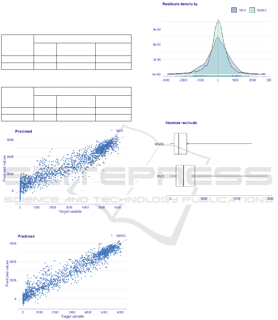
Table 2: Performance metrics: Training period
Machine
learning
algorithm
Training phase (20%)
𝑹
𝟐
𝑹𝑴𝑺𝑬 𝑲𝑾 𝑴𝑨𝑬 𝑲𝑾
MLR 0.8952 0.6852 0.5104
MARS 0.9413 0.5127 0.3699
Table 3: Performance metrics: Testing period
Machine
learning
algorithm
Testing phase (80%)
𝑹
𝟐
𝑹𝑴𝑺𝑬 𝑲𝑾 𝑴𝑨𝑬 𝑲𝑾
MLR 0.8987 0.6704 0.5054
MARS 0.9401 0.5155 0.3686
Figure 1: Predicted versus observed values plot – MLR
Figure 2: Predicted versus observed values plot – MARS
3.1.3 Residual Analysis
The residual analysis aims to check the accuracy of
regression models. Residuals, in general, represent
the portion of the target that the model is unable to
forecast. The following plot shows residual density
for MLR and MARS algorithms.
Figure 3: Residual density plot
The second plot represents the distribution of
residuals.
Figure 4: Residual boxplot
3.2 Discussion
Based on the results obtained in Tables 2 and 3, the
MARS approach demonstrated the best predictive
accuracy in terms of R²=94,01%, RMSE=0,5155Kw,
and MAE=0,3686Kw compared to MLR which
obtained R²=89,87%, RMSE=0,6704Kw, and
MAE=0,5054Kw in the testing phase.
Non-Linear algorithms tend to be more promising
than traditional regressions because they better
incorporate the dynamics of data and capture the non-
linear correlations between input and output
variables.
Furthermore, linear regression models are
incapable of capturing the non-linear structure of
independent variables, unlike the MARS algorithm,
which is considered as an advanced variant of
standard linear regression models.
Finally, residual analysis carried out in our study
shows that MARS surpasses MLR in predicting the
power produced by PV panels as we get a normally
Comparison of Machine Learning Techniques to Forecast the Output Power of Photovoltaic Panels using Multiple Prediction Factors
477

distributed residuals density that satisfies the
normality assumption of the residuals (Figure.3) and
residuals are close to zero (Figure.4)
4 CONCLUSIONS
In this article, we have used several input parameters
collected from internationally recognized sources to
predict the electrical power produced by PV panels.
We concluded that the MARS method demonstrated
superior accuracy than MLR in predicting the PV
power.
The results obtained also ensure the ability, with
high precision, of machine learning techniques to
forecast the PV power. In the likely future, these
algorithms will have a significant position in PV
remote management, where this technology will be
highly prevalent in several territories worldwide.
REFERENCES
S. Moslehi, T. A. Reddy, and S. Katipamula, “Evaluation
of data-driven models for predicting solar photovoltaic
power output,” Energy, vol. 142, pp. 1057–1065, 2018,
DOI: 10.1016/j.energy.2017.09.042.
I. Kaaya, S. Lindig, K. A. Weiss, A. Virtuani, M. Sidrach
de Cardona Ortin, and D. Moser, “Photovoltaic lifetime
forecast model based on degradation patterns,” Prog.
Photovoltaics Res. Appl., vol. 28, no. 10, pp. 979–992,
2020, DOI: 10.1002/pip.3280.
K. T. Dirk C. Jordan, Timothy J. Silverman, John H.
Wohlgemuth, Sarah R. Kurtz and VanSant,
“Photovoltaic failure and degradation modes,” Prog.
Photovoltaics Res. Appl., vol. 20, no. 1, pp. 6–11, 2017,
DOI: 10.1002/pip.2866.
S. Sobri, S. Koohi-Kamali, and N. A. Rahim, “Solar
photovoltaic generation forecasting methods: A
review,” Energy Convers. Manag., vol. 156, no. May
2017, pp. 459–497, 2018, DOI:
10.1016/j.enconman.2017.11.019.
N. Maitanova, J. Telle, B. Hanke, M. Grottke, T. Schmidt,
K. Von Maydell, C. Agert, “A machine learning
approach to low-cost photovoltaic power prediction
based on publicly available weather reports,” Energies,
vol. 13, no. 3, 2020, DOI: 10.3390/en13030735.
G. M. Spyros Theocharides, George E. Georghiou, Andreas
Kyprianou, “Machine Learning Algorithms for
Photovoltaic System Power Output Prediction,” 2018,
[Online]. Available: internal-
pdf://164.110.9.91/theocharides2018.pdf.
J. Wang, R. Ran, and Y. Zhou, “A short-term photovoltaic
power prediction model based on a FOS-ELM
algorithm,” Appl. Sci., vol. 7, no. 4, 2017, DOI:
10.3390/app7040423.
J. Antonanzas, N. Osorio, R. Escobar, R. Urraca, F. J.
Martinez-de-Pison, and F. Antonanzas-Torres,
“Review of photovoltaic power forecasting,” Sol.
Energy, vol. 136, pp. 78–111, 2016, DOI:
10.1016/j.solener.2016.06.069.
N. A. Ramli, M. F. A. Hamid, N. H. Azhan, and M. A. A.
S. Ishak, “Solar power generation prediction by using
the k-nearest neighbour method,” AIP Conf. Proc., vol.
2129, no. July, 2019, DOI: 10.1063/1.5118124.
A. Golder, J. Jneid, J. Zhao, and F. Bouffard, “Machine
learning-based demand and PV power forecasts,” 2019
IEEE Electr. Power Energy Conf. EPEC 2019, vol. 3,
2019, DOI: 10.1109/EPEC47565.2019.9074819.
M. Kayri, I. Kayri, and M. T. Gencoglu, “The performance
comparison of Multiple Linear Regression, Random
Forest and Artificial Neural Network using
photovoltaic and atmospheric data,” 2017 14th Int.
Conf. Eng. Mod. Electr. Syst. EMES 2017, pp. 1–4,
2017, DOI: 10.1109/EMES.2017.7980368.
B. Gschwind, L. Wald, P. Blanc, M. Lefèvre, M.
Schroedter-Homscheidt, and A. Arola, “Improving the
McClear model estimating the downwelling solar
radiation at ground level in cloud-free conditions -
McClear-v3,” Meteorol. Zeitschrift, vol. 28, no. 2, pp.
147–163, 2019, DOI: 10.1127/metz/2019/0946.
R. CoreTeam, R: A Language and Environment for
Statistical Computing, vol. 2. 2018.
Y. Li, Y. He, Y. Su, and L. Shu, “Forecasting the daily
power output of a grid-connected photovoltaic system
based on multivariate adaptive regression splines,”
Appl. Energy, vol. 180, pp. 392–401, 2016, DOI:
10.1016/j.apenergy.2016.07.052.
S. G. Kim, J. Y. Jung, and M. K. Sim, “A two-step approach
to solar power generation prediction based on weather
data using machine learning,” Sustain., vol. 11, no. 5,
2019, DOI: 10.3390/SU11051501.
BML 2021 - INTERNATIONAL CONFERENCE ON BIG DATA, MODELLING AND MACHINE LEARNING (BML’21)
478
