
Mathematical and Deep Learning Models Forecasting for
Hydrological Time Series
Lhoussaine El Mezouary
1
a
, Bouabid El Mansouri
2
b
and Samir Kabbaj
1
c
1
Laboratory of mathematical analysis, non-commutative geometry, and applications, Faculty of Science, Ibn Tofail
University, Campus Maamora, BP. 133 1400 Kenitra, Morocco Geosciences
2
Laboratory of hydroinformatics, Faculty of Sciences, University Ibn Tofail, Campus Maamora, BP. 133 1400 Kenitra,
Morocco
Keywords: hydrological forecasting, Deep learning, ANN, multilayer perceptron, backpropagation algorithm.
Abstract: Conventional hydrological models are based on a large number of readily accessible parameters. The use of
models with a small number of variables, cabals to treat the nonlinearity of these parameters is necessary.
With this in mind, we chose to develop a hydrological time series predictive model of flow based on the use
of Deep Learning models, the approach based on an ANN Method with a multilayer network without feedback
driven by the backpropagation algorithm errors. it is inspired by the principal mode of operation of the human
neurons with a function that transforms the activation response of non-linear type. The developed, unlike the
conventional statistical methods model, requires no assumptions on the variables used.
1 INTRODUCTION
The prediction of time series is the subject of several
studies in different fields and disciplines of research,
for example in biology and medicine, physics,
economics, and finance.
Over the past two decades, artificial neural
networks commonly used in applied physics have
entered management science as a quantitative method
of forecasting, alongside classical statistical methods
or by using direct parameters models equations (El
Mansouri and El Mezouary, 2015; El Mezouary,
2016; El Mezouary, El Mansouri, and El
Bouhaddioui, 2020; El Mezouary et al., 2015; El
Mezouary, El Mansouri, Moumen, et al., 2020; EL
MEZOUARY et al., 2016; Sadiki et al., 2019). They
are, in particular, used in hydrology, but other fields
of management are also concerned. There are
undoubtedly two main reasons which have led
researchers in Management Sciences to take an
interest in this tool (Aguilera et al., 2001; Ben-Daoud,
El Mahrad, et al., 2021; Ben-Daoud, Moumen, et al.,
2021; Huang et al., 2007).
a
https://orcid.org/0000-0000-0000-0000
b
https://orcid.org/0000-0000-0000-0000
c
https://orcid.org/0000-0000-0000-0000
The first is that, unlike classical statistical
methods, artificial neural networks do not require any
assumptions about the variables. The second is that
they are quite suitable for dealing with complex
unstructured problems, that is, problems on which it
is a priori impossible to specify the form of the
relationships between the variables used. It is through
algorithms that these systems learn on their own the
relationships between variables from a data set, much
like the human brain would. Thus, the network sets
itself up from the examples provided to it.
In recent years, several articles dealing with the
application of ANN to water resources management
have been published. One of the first applications was
that of forecasting water demand (Daniel and Chen,
1991), then neural networks were used for forecasting
water quality (Palani et al., 2008; Zhao et al., 2007)
and forecasting flow (Atiya et al., 1999; El Mezouary,
El Mansouri, and El Bouhaddioui, 2020).
In this article, we will first recall the notion of
hydrological forecasting and the models frequently
used, as well as various terms used in the context of
hydrological modeling. in the second place, we quote
the basic concepts and the development procedure of
El Mezouary, L., El Mansouri, B. and Kabbaj, S.
Mathematical and Deep Learning Models Forecasting for Hydrological Time Series.
DOI: 10.5220/0010732000003101
In Proceedings of the 2nd International Conference on Big Data, Modelling and Machine Learning (BML 2021), pages 249-254
ISBN: 978-989-758-559-3
Copyright
c
2022 by SCITEPRESS – Science and Technology Publications, Lda. All rights reserved
249

neural networks, their different structures, and their
learning algorithms. Finally, an application for a
hydrological forecast will present the characteristics
of phenomena and the result of the application of the
neural method to the forecasting of water river flows
and the discussion of the results.
2 PROBLEMS OF
HYDROLOGICAL
FORECASTING
The purpose of hydrological forecasts is to allow
more informed planning of interventions, as much for
flood or low water situations as in more common
hydrological conditions. Concerning the operation of
dams, forecasts make it possible to plan the opening
and closing of valves and spillways and thus help to
reduce the negative impacts linked to climatological
and hydrological hazards.
The purpose of ensemble hydrological forecasting
is to make available a set of forecasts at each time
step, so that this set allows the user to assess the
uncertainty of the forecast issued, depending on
whether the set covers a narrow or wide range of
values. When 𝑡 it means first run-through, the
computation of the anticipated streamflow 𝑄 at time
𝑡1 is of the accompanying structure:
𝑄
𝑄
𝑒̂
𝑓𝑄
,𝑋
,𝑒
( 1)
Where 𝑄
is the conjecture after 𝑙 time venture
forward, it compares to the measure of 𝑄
comparative with time 𝑡, 𝑋
is the network of
logical factors at time tl1, 𝑓 is the capacity
function of the valuation of 𝑄
and, 𝑒̂
is the
assessment of the calculated error 𝑒
.
It can be noted that the characteristic elements of
the forecast are:
The variable to predict and the explanatory
variables.
The forecast horizon (e.g., 𝐿 1 hour, 1 day, a
week, a month, a season, a year, return time ...).
Methods of calculation or estimation (i.e., the
nature of the function 𝑓.).
The objective of the forecast (flood warning,
planning of reservoir operation, irrigation, or
navigation projects).
The type of results desired (numeric values,
graphs, or probability distribution).
Taking all these elements into account in solving
Equation 1 constitutes "the problem of hydrological
forecasting", for medium and long-term forecasts, the
non-linear components of hydrometeorological
systems, and the number of explanatory variables
take on more importance (Coulibaly et al., 1999).
3 TIME-SERIES FORECASTING
Time series forecasting is a problem encountered in
several fields of application, such as finance
(prediction of future yield), engineering electricity
consumption), aeronautics (programming of
automatic pilots), etc. In hydrology (forecasting river
flows, forecasting of groundwater head, precipitation,
forecasting water quality....), the time series is a series
of ordered flow rates in time, where the instant
corresponding to the most recent element is
considered to be the present.
The goal is to predict one or more future elements
of the series. To achieve this, we must try to use as
much as possible the relevant information contained
in the time series itself, but also the information on
the possible influence of other time series (as for us
the one containing the precipitation data). Different
ways of using this information give rise to different
forecasting models.
Prediction models can be models characterized by
the degree of theoretical knowledge used regarding
the phenomenon under consideration or models that
use (almost) no theoretical knowledge. Models that
are not built entirely based on theoretical knowledge
are built from a learning set made up of observations
from the system. This set is so called because it
contains situations that the model can "learn" to
predict. after this learning phase, the forecasting
model has become capable of predicting situations
absent in the learning set, we speak of learning with
generalization.
The principal idea of forecasting is, time series
prediction models forecast values of a target data
𝑥
,
for a specified entity 𝑖
at
time 𝑡 (Lim and Zohren,
2021), any unit signifies a logical class of transient
data, example including measurements from
individual weather stations in climatology, and can be
observed at an equal time. inside the most effective
case, one-step-ahead forecasting models take the
form:
𝑥
,
𝑓𝑥
,:
,𝑦
,:
,𝑝
2
where
𝑥
,
is mean the hydrological model
forecast, the
𝑥
,:
,𝑦
,:
are represent the
target observations and exogenous inputs
BML 2021 - INTERNATIONAL CONFERENCE ON BIG DATA, MODELLING AND MACHINE LEARNING (BML’21)
250

respectively done a look-back case window 𝑘,𝑝
𝑖
is
stationary description data related to the entity, and
𝑓. is the estimate function learned by the time
series model. Similar components can be prolonged
to multivariate models (Lim and Zohren, 2021;
Salinas et al., 2019; Sen et al., 2019). A series of non-
linear layers are used to construct intermediate feature
representations (Bengio et al., 2013).
𝑓𝑥
,:
,𝑦
,:
,𝑝
ℎ
ℎ
𝑥
,:
,𝑦
,:
,𝑝
3
This equation is a basic Building Blocks of Deep
neural networks learn, were ℎ
and ℎ
are
respectively the encoder and decoder functions.
In Convolutional Neural Networks (CNNs), the
architecture is utilizing multiple layers of causal
convolutions (Bai et al., 2018; Borovykh et al., 2017)
to predict the time series datasets, each fundamental
convolutional filter takes the form of Equation 4 (Lim
and Zohren, 2021) below for an intermediate feature
at hidden layer 𝑙:
ℎ
𝐴
∑
𝑊
𝑙,𝜏
ℎ
4
For this convolutional architecture, the ℎ
is a
transitional at layer number one at time t, 𝑊
𝑙,𝜏
is a
weight of filter on layer 𝑙 . A. is a function of
activation, for example, sigmoid function,
representing any building and architecture-specific
non-linear processing. The recent modern
architectures make use of dilated convolutional layers
(Bai et al., 2018; Lim and Zohren, 2021), Equation 4
extend as below (Figure 1a):
𝑊∗ℎ𝑙,𝑡,𝑑
𝐴
∑
𝑊
𝑙,𝜏
/
ℎ
5
where 𝑑
𝜏 represent a layer-specific dilation rate.
The second architecture is Recurrent Neural
Networks, which assumed the normal interpretation
of time series data as inputs sequences data and
targets data, numerous RNN-based models have been
formed for transient estimating (Lim et al., 2019; Lim
and Zohren, 2021; Salinas et al., 2020). RNN cells
comprise an inward memory state which goes about
as a minimized past data rundown. For Elman RNN
(Elman, 1990), Figure 1b, the memory state is
recursively refreshed with novel perceptions at each
time project as displayed in the following condition:
𝑧
𝛾
𝑊
𝑧
𝑊
𝑦
𝑊
𝑥
𝑊
𝑠𝑏
6
Where 𝑧
∈ 𝑅
H is the RNN hidden internal
state. W is the linear weights, b is the biases of the
network, γ
are network activation functions.
The third architecture is Attention Mechanisms,
attention layers total transient highlights utilizing
progressively created weights displayed in Figure 1c,
permitting the network to straightforwardly zero in on
critical time steps before. Conceptually, attention is a
mechanism for a key-value lookup based on a given
query (Graves et al., 2014), taking the form below:
ℎ
∑
𝛼
𝑘
,𝑞
𝑣
7
Where intermediate features produced at different
time steps by lower levels of the network are the key
𝑘
, query 𝑞
and value 𝑣
. For time series
predicted, the attention gives two key advantages.
Initially, networks through attention can
straightforwardly go to any critical case that occurs.
Besides, as displayed in (Lim et al., 2021; Lim and
Zohren, 2021), attention-based networks can learn
regime-specific successive dynamics by using
separate attention weight designs for any regime.
The fourth basic Building Blocks of Deep neural
networks learn are Outputs and Loss Functions. In
one-step-ahead prediction problems (Lim and
Zohren, 2021). Forecasts can be further separated into
two different groups point estimates and probabilistic
predictions.
For Point Estimates, A typical way to deal with
estimating is to decide the normal worth of a future
objective. This includes reformulating the issue to a
characterization task for discrete outputs, and a
regression task for consistent outputs utilizing the
encoders portrayed previously (Lim and Zohren,
2021). Networks are qualified using binary cross-
entropy and mean square error loss functions
respectively in the case of one-step forward
predictions of binary and continuous targets. The
final layer of the decoder features a linear layer with
a sigmoid activation function allowing the network to
forecast the probability of event rate at a specified
time step in case of the binary classification:
𝑙
∑
𝑦
𝑙𝑜𝑔
𝑦
1 𝑦
log 1 𝑦
8
𝑙
∑
𝑦
𝑦
9
Mathematical and Deep Learning Models Forecasting for Hydrological Time Series
251
where 𝑙
, 𝑙
are the loss functions above are the most
common across applications, (Wen et al., 2017).
For Probabilistic Outputs, which use in some
applications, such as hydrological events, In the
presence of rare events, the full predictive distribution
will allow decision-makers to optimize their actions.
(Lim and Zohren, 2021). A common way to model
uncertainties is to use deep neural networks to
generate parameters of known distributions (Lim and
Zohren, 2021; Wen and Torkkola, 2019). For
forecasting problems with continuous targets,
Gaussian distributions are typically used, variance
parameters for the predictive distributions at each step
and networks outputting means as below(Lim and
Zohren, 2021):
𝑦
~𝑁𝑊
ℎ
𝑏
,𝑠𝑜𝑓𝑡𝑝𝑙𝑢𝑠𝑊
∑
ℎ
𝑏
∑
10
where the final layer of the network is represented by
ℎ
, function Softplus(.) means an activation function
to ensure that standard.
Figure 1: Different encoder architectures with temporal
information (Lim and Zohren, 2021)
4 RAINFALL-RUNOFF TIME
SERIES FORECASTING
MODEL
To proceed with the forecasting model, we start with
a preparation of a sufficient number of data to
constitute a representative base of the data likely to
occur during the use phase of the neural system. The
neural model is applied to daily rainfall (P) and flow
(Q) data from the river, the measurements cover a
period of 13 years. The average flow was of the order
2.67 m
3
/s, the maximum flow was 148 m
3
/s and the
minimum flow was 0.002 m
3
/s. Then the data was
subdivided into three, one to perform training, one for
validation, and another to test the resulting network.
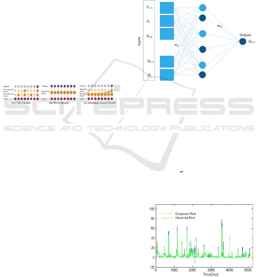
To predict the flow, we used the flow and rainfall
values observed at previous times t,t1,t2,t
3,... at the entrance to the network (Figure 2). The
network output represents the expected flow rate
Qt ∗ 1 for time t 1. With this assumption, a
structure of the RNN model can be expressed as:
𝑄
𝑅𝑁𝐴 𝑃
,𝑃
,𝑃
,𝑃
,
𝑄
,𝑄
,𝑄
11
However, to determine the input parameters that
participate and influence the output of the network,
we propose to test the neural network under different
scenarios. The calculation of the statistical parameters
allowed us to choose the best modelASE 2.
Figure 2: Model architecture
To detect and limit the overfitting of the model,
we will use the early stopping method. To select the
appropriate number of neurons in the hidden layer, we
vary the number of neurons in the hidden layer and at
the same time, we calculate the mean error of the ASE
squares of the test phase.
The best performing model is obtained for several
neurons equal to three in the hidden layer, which
corresponds to the minimum error of ASE =2.
𝐴𝑆𝐸
∑
𝑸
𝒊
𝑸
𝒊
𝟐
12
Where 𝑄
is the measured value of the flow, (𝑄
)
is the flow calculated by the model, N is the totality
of data of the calibration set.
Figure 3: calculated flows vs simulated flow rates
BML 2021 - INTERNATIONAL CONFERENCE ON BIG DATA, MODELLING AND MACHINE LEARNING (BML’21)
252

The model performance criteria for the learning
phase (Possess 70% of all data), the test phase
(Possess 15% of all data), and the validation phase
(Possess 15% of all data) are 0.23 for the ASE, and
0.83 for the 𝑅
, which is the coefficient of the
determination given by the below formula:
𝑅
2
1
∑
𝑄
𝑖
𝑄
𝑖
2
𝑁
𝑖1
∑
𝑄
𝑖
𝑄
𝑖
2
𝑁
𝑖1
13
Where 𝑄
𝑖
is the measured mean river flow. Figure
3 shows the calculated and simulated flow. It can be
seen that the flow values estimated by the network
follow the observed values. However, there are some
underestimations or overestimations, especially for
large flow values.
5 CONCLUSIONS
These results clearly show that artificial neural
networks can model the rainfall-discharge
relationship without the need to use parameters other
than precipitation and flow rate.
Neural networks can represent hydrologic time
series, even if they are complex and they are resistant
to noise or unreliable data. But the absence of a
systematic method allowing to define of the best
topology of the network and the number of neurons
to be placed in the hidden layers, the choice of the
initial values of the network weights, and the
adjustment of the learning step, which play an
important role in the speed of convergence and the
problem of overfitting remain the most important
drawbacks.
REFERENCES
Aguilera, P., Frenich, A. G., Torres, J., Castro, H., Vidal, J.
M., & Canton, M. J. W. r., 2001. Application of the
Kohonen neural network in coastal water management:
methodological development for the assessment and
prediction of water quality. 35(17), 4053-4062.
Atiya, A. F., El-Shoura, S. M., Shaheen, S. I., & El-Sherif,
M. S. J. I. T. o. n. n., 1999. A comparison between
neural-network forecasting techniques-case study: river
flow forecasting. 10(2), 402-409.
Bai, S., Kolter, J. Z., & Koltun, V. J. a. p. a., 2018. An
empirical evaluation of generic convolutional and
recurrent networks for sequence modeling.
Ben-Daoud, M., El Mahrad, B., Elhassnaoui, I., Moumen,
A., Sayad, A., ELbouhadioui, M., . . . Eljaafari, S. J. E.
C., 2021. Integrated water resources management: An
indicator framework for water management system
assessment in the R'Dom Sub-basin, Morocco. 3,
100062.
Ben-Daoud, M., Moumen, A., Sayad, A., ELbouhadioui,
M., Essahlaoui, A., & Eljaafari, S., 2021. Indicators of
Integrated Water Resources Management at the local
level: Meknes as a case (Morocco). Paper presented at
the E3S Web of Conferences.
Bengio, Y., Courville, A., Vincent, P. J. I. t. o. p. a., &
intelligence, m., 2013. Representation learning: A
review and new perspectives. 35(8), 1798-1828.
Borovykh, A., Bohte, S., & Oosterlee, C. W. J. a. p. a.,
2017. Conditional time series forecasting with
convolutional neural networks.
Coulibaly, P., Anctil, F., & Bobée, B. J. C. J. o. c. e., 1999.
Prévision hydrologique par réseaux de neurones
artificiels: état de l'art. 26(3), 293-304.
Daniel, A., & Chen, A. J. S. e., 1991. Stochastic simulation
and forecasting of hourly average wind speed
sequences in Jamaica. 46(1), 1-11.
El Mansouri, B., & El Mezouary, L. J. P. o. t. I. A. o. H. S.,
2015. Enhancement of groundwater potential by aquifer
artificial recharge techniques: an adaptation to climate
change. 366, 155-156.
El Mezouary, L., 2016. Modélisation mathématique et
numérique des phénomènes d’écoulements et de
transport de pollutions dans les milieux poreux:
application a l’aquifère alluvial de la rivière de Magra,
Italie.
El Mezouary, L., El Mansouri, B., & El Bouhaddioui, M.,
2020. Groundwater forecasting using a numerical flow
model coupled with machine learning model for
synthetic time series. Paper presented at the
Proceedings of the 4th Edition of International
Conference on Geo-IT and Water Resources 2020,
Geo-IT and Water Resources 2020.
El Mezouary, L., El Mansouri, B., Kabbaj, S., Scozzari, A.,
Doveri, M., Menichini, M., & Kili, M. J. L. H. B., 2015.
Modélisation numérique de la variation saisonnière de
la qualité des eaux souterraines de l'aquifère de Magra,
Italie. (2), 25-31.
El Mezouary, L., El Mansouri, B., Moumen, A., & El
Bouhaddioui, M., 2020. Coupling of numerical flow
model with the Susceptibility Index method (SI) to
assess the groundwater vulnerability to pollution. Paper
presented at the Proceedings of the 4th Edition of
International Conference on Geo-IT and Water
Resources 2020, Geo-IT and Water Resources 2020.
El Mezouary, L., Kabbaj, S., Elmansouri, B., Scozzari, A.,
Doveri, M., Menichini, M., . . . Applications. 2016.
Stochastic modeling of flow in porous media by Monte
Carlo simulation of permeability. 15.
Elman, J. L. J. C. s., 1990. Finding structure in time. 14(2),
179-211.
Graves, A., Wayne, G., & Danihelka, I. J. a. p. a., 2014.
Neural turing machines.
Huang, W., Lai, K. K., Nakamori, Y., Wang, S., Yu, L. J. I.
J. o. I. T., & Making, D., 2007. Neural networks in
finance and economics forecasting. 6(01), 113-140.
Lim, B., Arık, S. Ö., Loeff, N., & Pfister, T. J. I. J. o. F.,
2021. Temporal fusion transformers for interpretable
multi-horizon time series forecasting.
Mathematical and Deep Learning Models Forecasting for Hydrological Time Series
253

Lim, B., Zohren, S., & Roberts, S. J. a. p. a., 2019.
Recurrent neural filters: Learning independent
Bayesian filtering steps for time series prediction.
Lim, B., & Zohren, S. J. P. T. o. t. R. S. A., 2021. Time-
series forecasting with deep learning: a survey.
379(2194), 20200209.
Palani, S., Liong, S.-Y., & Tkalich, P. J. M. p. b., 2008. An
ANN application for water quality forecasting. 56(9),
1586-1597.
Sadiki, M. L., El-Mansouri, B., Benseddik, B., Chao, J.,
Kili, M., El-Mezouary, L. J. J. o. G. S., & Engineering.
2019. Improvement of groundwater resources potential
by artificial recharge technique: a case study of charf el
Akab aquifer in the Tangier region, Morocco. 7(3), 224-
236.
Salinas, D., Bohlke-Schneider, M., Callot, L., Medico, R.,
& Gasthaus, J. J. a. p. a., 2019. High-dimensional
multivariate forecasting with low-rank gaussian copula
processes.
Salinas, D., Flunkert, V., Gasthaus, J., & Januschowski, T.
J. I. J. o. F., 2020. DeepAR: Probabilistic forecasting
with autoregressive recurrent networks. 36(3), 1181-
1191.
Sen, R., Yu, H.-F., & Dhillon, I. J. a. p. a., 2019. Think
globally, act locally: A deep neural network approach
to high-dimensional time series forecasting.
Wen, R., Torkkola, K., Narayanaswamy, B., & Madeka, D.
J. a. p. a., 2017. A multi-horizon quantile recurrent
forecaster.
Wen, R., & Torkkola, K. J. a. p. a., 2019. Deep generative
quantile-copula models for probabilistic forecasting.
Zhao, Y., Nan, J., Cui, F.-y., & Guo, L. J. J. o. Z. U.-S. A.,
2007. Water quality forecast through application of BP
neural network at Yuqiao reservoir. 8(9), 1482-1487.
BML 2021 - INTERNATIONAL CONFERENCE ON BIG DATA, MODELLING AND MACHINE LEARNING (BML’21)
254
