Data Analysis within a Scientific Research Methodology

Fatima Ezzahra Chadli

, Driss Gretete

, Aniss Moumen

Engineering Sciences Laboratory, National School of Applied Sciences, Ibn Tofail University, Kenitra, Morocco

Keywords: Data analysis, scientific research methodology, statistical analysis, exploratory factor analysis, confirmatory

factor analysis.

Abstract: After identifying a problem, formulating a hypothesis, and developing a conceptual model, a crucial step

emerges in the researcher's approach towards collecting and analyzing data, which allows the use of statistical

techniques and the interpretation of data and results. This article sketch out the main steps of data analysis

within a scientific research methodology from a sampling strategy, to exploratory and confirmatory analysis.

1 INTRODUCTION

This paper focuses on two crucial steps in the

researcher’s approach; after identifying a problem,

formulating the hypothesis, and developing a

conceptual model, the next step is collecting and

analyzing data. It’s a process of gathering and

analyzing observations and measurements for

meaningful results. The approach, strategy and

techniques deployed during data collection and

analysis differ and depend on the researcher problem

and preferences.

This article sketch out the main steps of data

analysis, within a scientific research methodology,

from a sampling strategy to exploratory and

confirmatory analysis. Besides the literature review,

this paper summarizes a series of AOR workshops

about scientific research methodology and data

analysis organized by Dr Moumen Aniss, a professor

of computer science at the National School of

Applied Sciences-Kenitra.

2 SAMPLING STRATEGY

A sampling strategy impacts the quality of the data

collected; that’s why the researcher must adequately

identify the target population so that a sample would

be representative and reflect all its characteristics

(Taherdoost, 2016). The researcher can rely on the

https://orcid.org/0000-0001-5884-0350

https://orcid.org/0000-0001-8663-663X

https://orcid.org/0000-0001-5330-0136

literature review and the exploratory study to define

the target population's characteristics and the most

suitable sampling plan for the study.

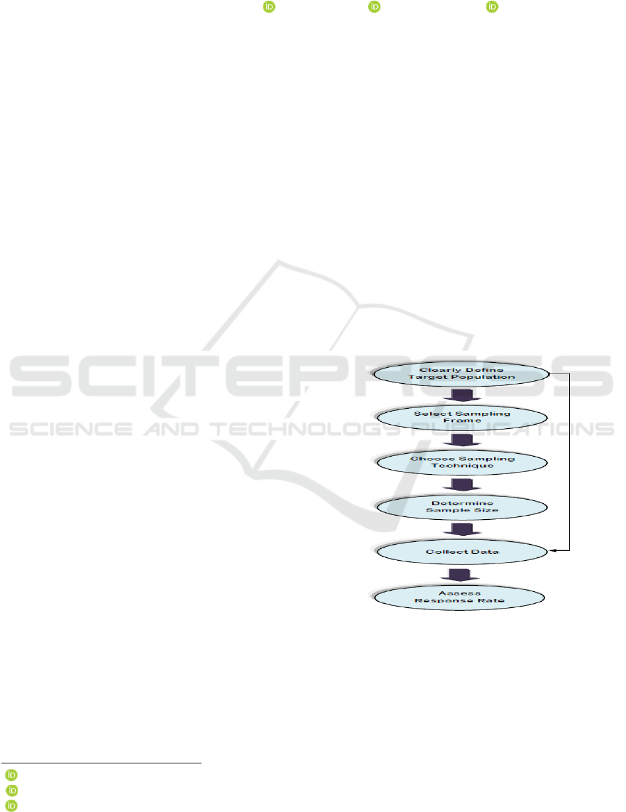
Figure 1 below shows steps of the sampling process

by (Taherdoost, 2016):

Figure 1: Sampling Process Steps by (Taherdoost, 2016)

2.1 Sampling Methods

Sampling methods differ depending on whether the

population is known or not; we talk about

probabilistic or non-probabilistic sampling

techniques (Moumen, 2019).

148

Chadli, F., Gretete, D. and Moumen, A.

Data Analysis within a Scientiﬁc Research Methodology.

DOI: 10.5220/0010730000003101

In Proceedings of the 2nd International Conference on Big Data, Modelling and Machine Learning (BML 2021), pages 148-153

ISBN: 978-989-758-559-3

According to (Taherdoost, 2016), in probability

sampling, the researcher selects individuals randomly

so that everyone has an equal chance to be chosen.

There are many types of probability sampling,

namely simple random, stratified random, cluster

sampling, systematic sampling and multistage

sampling. This category of sample ensures sufficient

representativity and reduces sampling bias risk.

In non-probability sampling, individuals are

selected based on non-random selection. A non-

probability sample includes quota sampling, snowball

sampling, judgement sampling, and convenience

sampling. This category of sample is the most

common among exploratory and qualitative research

(Taherdoost ,2016).

2.2 Sample Size

According to (Moumen, 2019), the determination of

the appropriate sample size is one of the frequent

problems in data analysis. It’s essential to consider

various factors when setting a sample size; the

researcher should identify the confidence interval,

margin of error, and confidence level.

The margin of error and the sample size are

inversely related; when the sample size increases, the

margin of error decreases (Moumen, 2019).

It’s essential to report the margin of error and the

confidence level to precise to what extent the results

could be generalized to the entire population.

Different statistical formulas are available for

calculating sample size and many calculators are

available online for this purpose (Moumen, 2019).

3 EXPLORATORY FACTOR

ANALYSIS

Factor analysis is a collection of methods that

examine how underlying constructs inﬂuence a set of

observed variables. There are two types of factor

analysis, namely exploratory and conﬁrmatory

analysis (DeCoster, 1998).

Exploratory factor analysis is a statistical

technique that explores the data collected and pre-tests

a measurement instrument; it focuses on reliability

and principal component analysis PCA tests

(Moumen, 2019).

It’s essential to emphasize the difference between

Principal Components Analysis (PCA) and

Exploratory Factor Analysis. According to (Costello

Osborne, 2005), there is a misconception caused by

two factors; the first is using PCA as the default

extraction technique in many statistical software, and

the second one uses PCA and EFA interchangeably.

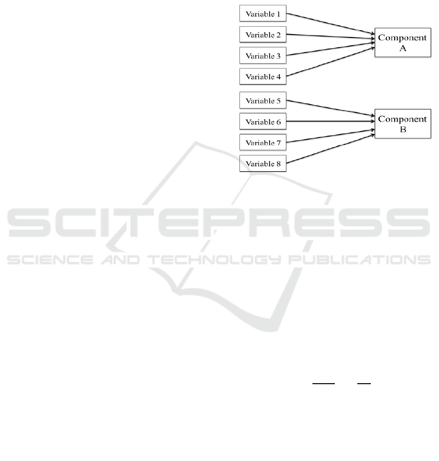
According to (Costello and Osborne, 2005), there

is a fundamental assumption made when choosing

PCA; the measured variables are themselves of

interest rather than some hypothetical latent construct

as in EFA. Figure 2 below shows a conceptual

overview of PCA.

Figure 2: Conceptual overview of Principal Components

Analysis by (Costello and Osborne, 2005)

3.1 Reliability of Measurement

After choosing or developing an instrument, the

researcher should pre-test this instrument, especially

for reliability consideration, which means to ensure

the extent to which the instrument can give the same

result after repeating the administration of the

instrument under stable conditions (Moser and

Kalton, 1989).

Cronbach's alpha is one of the most common

methods for checking the internal consistency of the

instrument.

Cronbach’s alpha formula:

𝜎=

𝑘

𝑘−1

1−

𝜎𝑖



𝜎







Where: k the number of items

σi² variance of ’item i

σt² total score variance

(Hinton et al., 2004) have suggested four cut-off

points for reliability; excellent reliability (0.90 and

above), high reliability (0.70-0.90), moderate

reliability (0.50-0.70) and low reliability (0.50 and

below) (Hinton et al., 2004).

The researcher can apply Cronbach’s alpha in the

case of One-dimensional Exploratory Analysis. For

the possibility of multidimensional exploratory

Data Analysis within a Scientiﬁc Research Methodology

149

analysis, principal component analysis (PCA) is

recommended with Kaiser-Meyer-Olkin (KMO) and

Bartlett’s methods.

3.2 Suitability of Data for Factor

Analysis

There are two conditions to check that the observed

data is suitable and appropriate for exploratory factor

analysis; Sampling Adequacy tested by The Kaiser-

Meyer-Olkin KMO. The relationship among

variables is assessed through Bartlett’s test sphericity

(Moumen, 2019).

3.2.1 Kaiser-Meyer-Olkin KMO

The KMO method measures the adequacy of the

sample; if the value of the KMO is more than 0.5, the

sampling is sufficient; according to (Kaiser, 1974),

A high KMO indicates that there is a statistically

acceptable factor solution.

3.2.2 Bartlett Test of Sphericity

The researcher uses the Bartlett test of Sphericity to

check if there is redundancy among variables that

could be summarized with a few factors, in other

words, to verify data compression in a meaningful

way. This test comes before data reduction techniques

such as principal component analysis (PCA)

(Gorsuch, 1973).

4 CONFIRMATORY FACTOR

ANALYSIS

EFA explores whether your data fits a model that

makes sense based on a conceptual or theoretical

framework. It doesn’t confirm hypotheses or test

competing models as in confirmatory factor analysis

CFA (Costello and Osborne, 2005).

According to (Hoyle, 2012) CFA is a multivariate

statistical procedure for testing hypotheses about the

commonality among variables.

Confirmatory factor analysis concerns a large

sample that exceeds 30 observations according to

Gaussian law; this analysis aims to prove or disprove

the research hypotheses (Moumen, 2021).

4.1 Hypothesis Testing

The hypothesis testing evaluates what data provides

against the hypothesis. The researcher begins a test

with two hypotheses called the null hypothesis H0

and the alternative hypothesis H1, and the two

hypotheses are opposite (Moumen, 2021).

If data provides enough evidence against the

hypothesis, it will be rejected. To reject or accept the

null hypothesis H0, there is a Significance Level

(Alpha) beyond which we cannot reject the null

hypothesis. Alpha is the probability that a researcher

make a mistake of rejecting the null hypothesis that

is, in fact, true (Moumen, 2021).

Three options are available for a significance

level: 5%, 1% and 0.1%; the choice of a significance

level is conventional and depends on the field of

application. (Moumen, 2021).

A golden rule for a significance level of 5%

(Moumen, 2021):

If alpha > 5%, H0 is accepted, and H1 is rejected. If

alpha <= 5%, then H0 is rejected, and H1 is accepted.

Examples of statistical hypotheses:

- Normal distribution hypothesis

- Representativeness test

- Test of association

There are two categories of hypothesis testing;

parametric and non-parametric hypothesis (Verma,

2019).

4.1.1 Parametric Hypothesis Test

According to (Verma, 2019), the parametric tests aim

to test the adequacy of the observed distribution of the

random variables on the sample compared to the

known and pre-established (supposed) statistical

distribution of the population.

The goal is to compare the parameters observed

with the theoretical parameters to generalize from the

sample to the population, with a margin of error.

The parametric hypothesis test supposes a normal

distribution of values (Verma, 2019).

Examples of parametric tests:

-Chi-square

-One-Way Anova

- Simple t-test

4.1.2 Non-parametric Hypothesis Test

The researcher can use non-parametric tests when

parametric tests are not appropriate. It doesn’t require

any assumption on the statistical distribution of data

and doesn’t involve population parameters (Datta,

2018).

The purpose of this test remains the same as the

parametric tests; that means to verify the hypothesis

according to a Significance Level (Alpha).

BML 2021 - INTERNATIONAL CONFERENCE ON BIG DATA, MODELLING AND MACHINE LEARNING (BML’21)

150

Those tests are more suitable for small samples (<30)

and when the variables are more qualitative: Nominal

and Ordinal (Datta, 2018).

Examples of non-parametric tests:

- Chi-square

- Wilcoxon signed-rank test

- Kruskal

- Wallis test

4.2 Statistical Modelling

According to (Retherford, 2011), statistical

modelling enables the researcher to understand how a

phenomenon evolves depending on a set of

parameters; it’s a simplified representation to

understand reality or even make predictions.

Technically how does it work? A model explains a

dependant or measured variable by an independent

variable via mathematical equations involving

parameters.

4.2.1 Simple Linear Regression

Simple linear regression is a statistical method used

to analyze a relationship between two variables; an

independent variable pointed x, and a dependent

variable pointed y (Retherford, 2011).

The form of the simple linear regression equation is:

Y= a + bX + ε

Where: Y is the dependent variable

X is the independent variable

a is the y-intercept.

b is the slope of the line

ε is the residual or the error that the model

couldn’t explain.

It’s essential to distinguish between regression and

correlation; regression

attempts to establish a

mathematical model of the relationship between a

dependent and independent variable to predict a

dependent variable when the independent variable is

known.

While correlation is an evaluation of this

relationship (does it exist or not), the strength of that

relation (is it strong or weak) and the sign of the

correlation coefficient (positive or negative).

Correlation is a prerequisite for regression (Shi,

2009).

According to (Moumen, 2021), simple linear

regression requires the following condition to be

verified:

-The two variables are continuous

-The relationship between the two variables is

approximately linear.

-There are no or few aberrant values.

-The residual is independent of X and follow a normal

distribution

-The variance of Y is the same for all values of X

(Homoscedasticity)

4.2.2 Multiple Linear Regression

According to (Moumen, 2021), multiple linear

regression is a statistical method used to analyze a

relationship between a dependent variable and two or

multiple independent variables.

The form of the simple linear regression equation is:

Y= a + b1X1 + b2X2+…+ ε

Multiple linear regression requires the following

condition to be verified (Moumen, 2021):

-Variables are continuous.

-The relationship between variables is approximately

linear

- No aberrant values

-The residual is independent of Y and follow a normal

distribution

-The variance of Y is the same for all values of X

(homoscedasticity)

-No multicollinearity (no correlation between

independent variables X)

4.2.3 Logistic Regression

Logistic regression is one technique used to analyze a

relationship between dependent and one or more

independent variables. When the type of independent

variable is qualitative, logistic regression is adequate

(Moumen, 2021).

There are three types of logistic regression

(Moumen, 2021):

-Binary Logistic Regression is used in the case where

the dependent variable has two modalities.

- Multinomial Logistic Regression is used when the

dependent variables have more than two modalities

and are not ordinal.

-Ordinal Logistic Regression is used when the

dependent variables have more than two modalities

and are ordinal.

4.2.4 Structural Equation Modelling

Structural equation modelling SEM also known as

covariance structure is a multivariate statistical

analysis technique. It’s not one statistical technique

but a set of techniques that integrates measurement

theory, factor analysis (latent variable) and regression

(Stein, Morris, et Nock, 2012).

In regression models, there is one dependent

variable and a set of predictors or independent

variables. In a structural equation model, there are

Data Analysis within a Scientiﬁc Research Methodology

151

Numerous dependent variables, each of which is in

relation with other dependent variables, which create

a complex system and allows a researcher to test a set

of regression equations simultaneously (Stein,

Morris, et Nock, 2012).

The researcher can use structural equation

modelling for indirect and direct effects of variables

on other variables (the case of mediated research

questions).

Modelisation represents a path diagram that shows

the interconnection between variables indicating a

causal flow. The diagram integrates latent variables

as ovals and boxes for independent or manifest

variables (Moumen, 2021).

There are two components of structural equation

modelling: a measurement model for manifest

variables and a structural model for latent variables

(Moumen, 2021).

There are many software packages for structural

equation modelling; the more known are LISREL,

AMOS, and R. This article will focus on Amos

software.

4.2.5 Structural Equation Modeling using

AMOS

Many visual SEM software help to design the

theoretical models graphically using simple drawing

tools. It can also estimate the model’s fit and give a

final valid model (N. et Rajendran, 2015).

Analysis of Moment Structures or AMOS is statistical

software analyzing a moment structure or structural

equation modelling. It’s an SPSS module that extends

multivariate analysis methods like regression and

factor analysis and includes a set of statistical features

for all analytical processes from data preparation to

analysis (Barnidge, 2017).

There are six main steps to follow for structural

equation modelling with AMOS (Moumen, 2021):

Table 1: SEM steps with AMOS.

Step SPSS

STATISTICS

AMOS

extract factors

✓

verify reliability

✓

Discriminant validity

✓

test the first-order

factor

✓

test a second-order

factor

✓

test mediation effects

✓

According to (Arbuckle, 2018), Amos is User-

friendly software with simple drawing tools to

manage models graphically and display parameter

estimates on a path diagram.

Below description of basic steps using Amos graphics

23.0.0 (Arbuckle, 2018) IBM® SPSS® Amos™ 23

User’s Guide:

-Create a new Model: to start researcher has to draw

a path diagram using a toolbar; many features are

available.

-Specify the Data File: next step is to import data;

Amos supports several file formats like SPSS file

extension; the user needs to specify the types of file

to import under the type list.

-Specify variables: after specifying the data, the next

step is to associate each variable in the dataset to its

rectangle. For residuals, Amos provides a plugin

module that assigns names to unobserved variables.

-Identify a model: before start calculating, it’s

necessary to identify a model by specifying a latent

variable.

-Calculate estimation: to calculate estimation Amos

provides a simple function under analysis; the output

window gives interesting indicators; the first one is

chi-square that measures the extent to which the

model is compatible with the hypothesis, and the

second one is probability level.

5 CONCLUSIONS

Exploratory factor analysis EFA provides insights

into the dimensionality of the latent variables and

confirms the reliability of the measurement. EFA

gives preliminary factor structure of constructs, while

confirmatory factor analysis CFA determines the

validity of the measures and the construct validity.

The researcher should have some basics about

theoretical concepts to ensure that items measure the

construct. The literature review and the exploratory

study plays an important role to define the

characteristics of the target population and the

sampling plan; the more the population and the

concepts are mastered, the more the data collected is

reliable, and the results are meaningful.

REFERENCES

Taherdoost, Hamed. 2016. « Sampling Methods in

Research Methodology; How to Choose a Sampling

Technique for Research ». International Journal of

Academic Research in Management Vol.5, page:

18‑27. https://doi.org/10.2139/ssrn.3205035.

BML 2021 - INTERNATIONAL CONFERENCE ON BIG DATA, MODELLING AND MACHINE LEARNING (BML’21)

152

Aniss Moumen 2019, “AOR workshop sur l’élaboration du

questionnaire, échantillonnage et Analyse factorielle

exploratoire avec SPSS”.

DeCoster, Jamie. 1998. « Overview of Factor Analysis »

Costello, AB, et Jason Osborne. 2005. « Best Practices in

Exploratory Factor Analysis: Four Recommendations

for Getting the Most From Your Analysis ». Practical

Assessment, Research & Evaluation 10: 1‑9.

Moser, Claus, et Graham Kalton. 1989. Survey Methods in

Social Investigation. London: Gower.

Dr Perry Hinton, Perry R. Hinton, Isabella McMurray, et

Charlotte Brownlow. 2004. SPSS Explained.

Routledge.

Kaiser, Henry F. 1974. « An Index of Factorial Simplicity

». Psychometrika 39 (1): 31‑36.

https://doi.org/10.1007/BF02291575.

Gorsuch, Richard L. 1973. « Using Bartlett’s Significance

Test to Determine the Number of Factors to Extract ».

Educational and Psychological Measurement 33 (2):

361‑64. https://doi.org/10.1177/001316447303300216.

Hoyle, Rick. 2012. « Confirmatory Factor Analysis ».

Handbook of Applied Multivariate Statistics and

Mathematical Modeling, October.

https://doi.org/10.1016/B978-012691360-6/50017-3.

Aniss Moumen, 2021 “AOR workshop sur l’analyse

factorielle confirmatoire avec SPSS Tests d'hypothèse

Régression Classification”.

Verma, J. P., et Abdel-Salam G. Abdel-Salam. 2019.

Testing Statistical Assumptions in Research. John

Wiley & Sons.

Datta, Sanjoy. 2018. Concept of Non-parametric Statistics.

https://doi.org/10.13140/RG.2.2.18033.12648.

Retherford, Robert D., et Minja Kim Choe. 2011. Statistical

Models for Causal Analysis. John Wiley & Sons.

Shi, Runhua, et Steven Conrad. 2009. « Correlation and

regression analysis ». Ann Allergy Asthma Immunol

103: S35-41.

Stein, Catherine, Nathan Morris, et Nora Nock. 2012. «

Structural Equation Modeling ». Methods in molecular

biology (Clifton, N.J.) 850 (Janvier): 495‑512.

https://doi.org/10.1007/978-1-61779-555-8_27.

N., Elangovan, et Raju Rajendran. 2015. « Structural

equation modeling-A second-generation multivariate

analysis ».

Barnidge, Matthew, et Homero Gil de Zúñiga. 2017, «

Amos (Software) »

https://doi.org/10.1002/9781118901731.iecrm0003.

Arbuckle, James L. s. d. 2018 « IBM® SPSS® Amos

User’s Guide », 702.

Data Analysis within a Scientiﬁc Research Methodology

153