Analytical Solution of Homogeneous Groundwater Flow Equation

using Method of Separation of Variables

Lhoussaine El Mezouary

, Samir Kabbaj

and Bouabid El Mansouri

Laboratory of mathematical analysis, non-commutative geometry, and applications, Faculty of Science, Ibn Tofail

University, Campus Maamora, BP. 133 1400 Kenitra, Morocco Geosciences

Laboratory of Natural Resources, hydroinformatics Team, Faculty of Sciences, University Ibn Tofail, Campus Maamora,

BP. 133 1400 Kenitra, Morocco

Keywords: Method of Separation of Variables, Groundwater Equation, Diffusion Equation, Porous Media, heat diffusion

equation.

Abstract: This paper presents an analytical solution for predicting the one-dimensional (1D) time-dependent

groundwater flow profile in an unconfined system. This hydraulic charge prediction problem is modeled as a

boundary value problem governed by the heat diffusion equations. The solution technic employs the

separation of variables method, the results are compared to the numerical solution, and the solution displays

a reasonable flow head during different periods.

1 INTRODUCTION

The groundwater equation governed through Darcy

law and the continuity equation was the subject of a

set of research. Among the first researchers

concerned with this equation (Bansal and Das, 2011;

Bear, 2013; Chapman, 1980; Childs, 1971; Glover,

1960; Hantush, 1967; McDowell‐Boyer et al., 1986;

Simmons et al., 2001; Verhoest and Troch, 2000;

Wooding and Chapman, 1966). Initially, these

researches focused on trying to understand the

behavior of groundwater and its flow mechanisms in

porous media. These researches have focused to find

solutions to the groundwater equation, the researchers

analyzed the mechanisms of evolution and regular

groundwater flow regeneration in the aquifers. as a

result, it has been proposed and developed a set of

analytical solutions (Manglik et al., 1997; Pauwels et

al., 2002; Rai and Manglik, 1999; Verhoest and

Troch, 2000).

In the same context, some recherche has focused on

finding in obtaining analytical solutions to the linear

Boussinesq equation by adopting the uniform

recharge of the rainfall rate, therefore these solutions

https://orcid.org/0000-0000-0000-0000

are exploited to estimate the groundwater levels

change and drainage flow (Pauwels et al., 2002;

Serrano, 1995; Verhoest and Troch, 2000).

Other research focused on researching analytical

solutions for the same equation, taking into account

the hypothesis of temporal variation of the level of

rainfall (Dralle et al., 2014; Park and Parker, 2008;

Pauwels et al., 2002; Ram and Chauhan, 1987; Su,

1994; Thomas, 2013).

Some other research has worked on the Laplace

Transform method to develop an analytical solution

to express the distribution of groundwater levels

(Bansal and Das, 2011; Kim and Ann, 2001; Kumar

et al., 2016; Pauwels et al., 2002; Sun et al., 2011).

On the other hand, special studies have worked on

the use of some numerical solutions as a mechanism

for studying and developing models of groundwater

flow equation (Draoui et al.; El Mansouri and El

Mezouary, 2015; El Mezouary, 2016; El Mezouary,

El Mansouri, and El Bouhaddioui, 2020; El Mezouary

et al., 2015; El Mezouary, El Mansouri, Moumen, et

al., 2020; EL MEZOUARY et al., 2016; Sadiki et al.,

2019) as a model of forecasting and simulating the

dynamic behavior based on boundary conditions.

El Mezouary, L., Kabbaj, S. and El Mansouri, B.

Analytical Solution of Homogeneous Groundwater Flow Equation using Method of Separation of Variables.

DOI: 10.5220/0010729900003101

In Proceedings of the 2nd International Conference on Big Data, Modelling and Machine Learning (BML 2021), pages 143-147

ISBN: 978-989-758-559-3

143

The present study focused on the method of

Separation of Variables for solving the groundwater

equation using Darcy’s law as a theoretical basis and

applied the principle of mass conservation (the

continuity equation) to govern the groundwater flow.

2 GROUNDWATER FLOW

EQUATION

The general groundwater flow equation is deducted

from Darcy’s law and the continuity equation. The net

rate of penetration of a fluid in a control volume is

exactly equal to the net rate of change of storage of

the mass of fluid in the same control volume.

We begin by examining the last groundwater flow

phenomena (Diffusion), which are treated similarly

with a linear diffusion partial differential equation.





𝐾







ℎ

(

𝑥,𝑦,𝑧,𝑡

)

+





𝐾







ℎ

(

𝑥,𝑦,𝑧,𝑡

)

+





𝐾







ℎ

(

𝑥,𝑦,𝑧,𝑡

)

=𝑆







ℎ

(

𝑥,𝑦,𝑧,𝑡

)

−

𝑞

(

𝑥,𝑦,𝑧,𝑡

)

(1)

Where 𝐾



, 𝐾



, 𝐾



are the hydraulic conductivity,

𝑆



is specific storage, ℎ is the piezometric head.

We consider the equations in one dimension that

the medium is uniform. which means that the

coefficient of permeability 𝐾 is spatially invariant,

we can write to them as simple constants. Then,

equation 1 is simplified by:

𝑘(

𝜕



𝜕𝑥



ℎ(𝑥,𝑡))=

𝜕ℎ(𝑥,𝑡)

𝜕𝑡

(2)

Where 𝑘is the groundwater flow diffusivity or

hydraulic diffusivity of the medium, are 𝐿



/T:

𝑘=

𝐾

𝑆



(3)

3 ANALYTICAL SOLUTION

In this level, we will proceed to solve the groundwater

flow equation 2 by the variable separation method:

We note that 𝑥 represents the position in the one-

dimensional medium (an aquifer) that we can identify

with the interval [0,𝐿]. The hydraulic height in this

aquifer at time 𝑡 and location 𝑥 is ℎ(𝑥,𝑡).

A typical problem is to consider that the

distribution of the hydraulic height over the entire

length of the aquifer is known at time 𝑡=0 (initial

condition) and that the flow of groundwater through

the ends 𝑥=0 and 𝑥=𝐿 are given values (boundary

conditions). Therefore we can imagine that the

hydraulic height is determined for 𝑥∈(0,𝐿) and 𝑡>

0. The conditions imposed on the ends are often of

the form:

- ℎ(0,𝑡)= 0 or,

(,)



=0 or

(,)



=0=

𝑎ℎ(0,𝑡)

- ℎ(𝐿,𝑡) =0 or,

(,)



=0 or

(,)



=0=

−𝑎ℎ(𝐿,𝑡)

Where 𝑎>0 is also a physical constant. The

solution of problem (2) given by the method of

separation of variable it is as follows:

ℎ(𝑥,𝑡)=

∑

𝑠𝑖𝑛











|







/

𝑥



𝑄



𝑒







(4)

Since 𝜆



=−𝑘(𝑛+





)













the equation can be

written in this formula:

ℎ(𝑥,𝑡)=𝑠𝑖𝑛









(

𝛼𝜋𝑥

)

𝑄



𝑒



[



]





(5)

Where 𝛼=

(



)



, and the 𝑄



is:

𝑄









𝑠𝑖𝑛







(

𝛽

)

/

𝑥𝜑(𝑥)𝑑𝑥,∀𝑛 ∈ ℕ (6)

Where 𝛽=

|





, 𝑄



also can be written :

𝑄









𝑠𝑖𝑛





(𝛼𝜋𝑥)𝜑(𝑥)𝑑𝑥 (7)

4 SIMULATION OF SOLUTION

Consider the case of a 1𝐷 flow problem on an

unconfined aquifer that a river and a lake run parallel

to each other (figure 1) with 𝐿=500𝑚 apart. They

fully penetrate aquifer with a hydraulic conductivity

𝐾=400 𝑚/𝑑𝑎𝑦, and specific yield 𝑆



=22%. To

demonstrates the feasibility of the analytical solution

given by method of separation of variable, we are

compared it by a two numerical profile simulated

using the CrankNicholson implicit method

(

)

BML 2021 - INTERNATIONAL CONFERENCE ON BIG DATA, MODELLING AND MACHINE LEARNING (BML’21)

144

(Thomas, 2013) and the Forward Time Centered

Space method (FTCS)

(

)

(Anderson et al., 1997).

The CrankNicholson implicit method consists of

replacing the second derivative











in the equation

(

)

by the average of its discrete representations at

times 𝑛 and 𝑛+1.































(

ℎ





−2ℎ





+ℎ





)





(

ℎ





−2ℎ





+ℎ





)

 (8)

While for the Forward Time Centered Space

(FTCS) or forward/backward space method is an

implicit single-stage finite difference method that can

use for numerically solving the heat equation and

similar parabolic partial differential equations.

This scheme is unconditionally stable. then the

equation

(

)

can be represented by the flowing

scheme:

ℎ





=ℎ





+𝛼

(

ℎ





−2ℎ





+ℎ





)

(9)

With 𝛼=







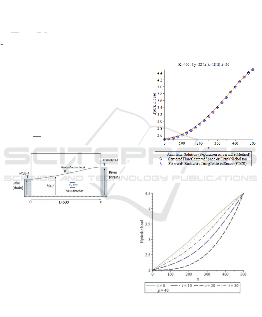
Figure 1: Groundwater flow conceptual model on

unconfined, horizontal aquifer with dirichlet boundary

condition

This solution example corresponds to the

following mathematical problem with

nonhomogeneous Dirichlet boundary conditions

(Figure 2).

⎩

⎪

⎨

⎪

⎧

𝑘

𝜕



𝜕𝑥



ℎ

(

𝑥,𝑡

)

=

𝜕ℎ

(

𝑥,𝑡

)

𝜕𝑡

0𝑥𝐿,𝑎𝑛𝑑 0𝑡𝑇;

ℎ(0,𝑡)=2,ℎ(𝐿,𝑡)=4.5, 0𝑡𝑇;

ℎ(𝑥,0)=(2+

𝑥



510



), 0𝑥𝐿

(10)

Following the solution represented by equation 4,

the simulation of the solution illustrate on problem

(

)

is shown in Figure 2, the figure show

comparison

of the evaluated exact solution with implicit numerical

methods of CrankNicholson

and FTCS, while Figure 3

shows the evaluated exact solution at various times

𝑡=10,𝑡=20,𝑡=30,𝑡=40.

It should be remembered that this simulation took

into account the imposed boundary conditions, based

on the conceptual model shown in Figure 1, it is

obvious that the figure's results provide a good match

solution at different times.

Figure 2: Comparison of the evaluated exact solution with

implicit numerical methods of CrankNicholson and FTCS.

Figure 3: evaluated exact solution at various times.

Analytical Solution of Homogeneous Groundwater Flow Equation using Method of Separation of Variables

145

5 DISCUSSION

Analytical solution for the prediction of the one-

dimensional (1𝐷) time-dependent groundwater flow

profile in an unconfined system evaluated for a

setting corresponding case to 𝐿=500 𝑚, K=

400 m, k=1818 𝑚



/d, 𝑆



=22%. The solution

uses a uniform domain in different time step lengths.

The simulation results obtained according to equation

4, the results showing note that the solution produced

by the method of separation of the variable is

acceptable, as well as that in all the cases in which the

solution was applied, it was found that there is a

match between the solution produced by the

separation of variable method and with the other two

numerical methods of CrankNicholson and FTCS

method.

The module can simulate the same solutions that

were given by the CrankNicholson and FTCS

methods. It can then be concluded that the solution is

given by the separation of the variable method when

applied in a homogeneous medium, taking into

account the normal boundary conditions, the solution

presented can reproduce the behavior of the

groundwater in a very acceptable way.

6 CONCLUSIONS

The paper introduces an analytical solution of a one-

dimensional groundwater equation for a homogenous

porous media. Using the method of separation of

variables, this solution precisely reproduces the

similar solution given from CrankNicholson and

FTCS finite-difference methods. An example is used

to verify the proposed solution, considering constant

head in boundary conditions (Dirichlet conditions).

The analytical solution has been compared with the

CrankNicholson and FTCS numerical solutions, for a

context with sand-gravel medium characteristics. The

correlation is good within the example case. In

consequence, the proposed method is valid for the

homogenous horizontal unconfined aquifer, also for

another similar physical or environmental problem.

REFERENCES

Anderson, D. A., Tannehill, J. C., & Pletcher, R. H. (1997).

Computational fluid mechanics and heat transfer:

Taylor & Francis.

Bansal, R. K., & Das, S. K. J. W. r. m., 2011. Response of

an unconfined sloping aquifer to constant recharge and

seepage from the stream of varying water level. 25(3),

893-911.

Bear, J. (2013). Dynamics of fluids in porous media:

Courier Corporation.

Chapman, T. J. W. R. R., 1980. Modeling groundwater flow

over sloping beds. 16(6), 1114-1118.

Childs, E. J. W. R. R., 1971. Drainage of groundwater

resting on a sloping bed. 7(5), 1256-1263.

Dralle, D. N., Boisramé, G. F., & Thompson, S. E. J. W. R.

R., 2014. Spatially variable water table recharge and the

hillslope hydrologic response: Analytical solutions to

the linearized hillslope Boussinesq equation. 50(11),

8515-8530.

Draoui, Y., Lahlou, F., Chao, J., El Mezouary, L., Al

Mazini, I., & El Hamidi, M. J., Quantification of

Surface Water-Groundwater Exchanges by GIS

Coupled with Experimental Gauging in an Alluvial

Environment.

El Mansouri, B., & El Mezouary, L. J. P. o. t. I. A. o. H. S.,

2015. Enhancement of groundwater potential by aquifer

artificial recharge techniques: an adaptation to climate

change. 366, 155-156.

El Mezouary, L., 2016. Modélisation mathématique et

numérique des phénomènes d’écoulements et de

transport de pollutions dans les milieux poreux:

application a l’aquifère alluvial de la rivière de Magra,

Italie.

El Mezouary, L., El Mansouri, B., & El Bouhaddioui, M.,

2020. Groundwater forecasting using a numerical flow

model coupled with machine learning model for

synthetic time series. Paper presented at the

Proceedings of the 4th Edition of International

Conference on Geo-IT and Water Resources 2020,

Geo-IT and Water Resources 2020.

El Mezouary, L., El Mansouri, B., Kabbaj, S., Scozzari, A.,

Doveri, M., Menichini, M., & Kili, M. J. L. H. B., 2015.

Modélisation numérique de la variation saisonnière de

la qualité des eaux souterraines de l'aquifère de Magra,

Italie. (2), 25-31.

El Mezouary, L., El Mansouri, B., Moumen, A., & El

Bouhaddioui, M., 2020. Coupling of numerical flow

model with the Susceptibility Index method (SI) to

assess the groundwater vulnerability to pollution. Paper

presented at the Proceedings of the 4th Edition of

International Conference on Geo-IT and Water

Resources 2020, Geo-IT and Water Resources 2020.

El Mezouary, L., Kabbaj, S., Elmansouri, B., Scozzari, A.,

Doveri, M., menichini, m., . . . Applications. 2016.

Stochastic modeling of flow in porous media by Monte

Carlo simulation of permeability. 15.

Glover, R. J. A. R. S., Ft. Collins, Colo., 1960.

Mathematical derivations pertaining to groundwater

recharge, US Dept. Agr.

Hantush, M. S. J. W. R. R., 1967. Growth and decay of

groundwater ‐ mounds in response to uniform

percolation. 3(1), 227-234.

Kim, D. J., & Ann, M. J. J. H. P., 2001. Analytical solutions

of water table variation in a horizontal unconfined

aquifer: Constant recharge and bounded by parallel

streams. 15(13), 2691-2699.

BML 2021 - INTERNATIONAL CONFERENCE ON BIG DATA, MODELLING AND MACHINE LEARNING (BML’21)

146

Kumar, S., Kumar, A., & Baleanu, D. J. N. D., 2016. Two

analytical methods for time-fractional nonlinear

coupled Boussinesq–Burger’s equations arise in

propagation of shallow water waves. 85(2), 699-715.

Manglik, A., Rai, S., & Singh, R. J. W. r. m., 1997.

Response of an unconfined aquifer induced by time

varying recharge from a rectangular basin. 11(3), 185-

196.

McDowell‐Boyer, L. M., Hunt, J. R., & Sitar, N. J. W. r.

r., 1986. Particle transport through porous media.

22(13), 1901-1921.

Park, E., & Parker, J. J. J. o. H., 2008. A simple model for

water table fluctuations in response to precipitation.

356(3-4), 344-349.

Pauwels, V. R., Verhoest, N. E., & De Troch, F. P. J. W. R.

R., 2002. A metahillslope model based on an analytical

solution to a linearized Boussinesq equation for

temporally variable recharge rates. 38(12), 33-31-33-

14.

Rai, S., & Manglik, A. J. J. o. H., 1999. Modelling of water

table variation in response to time-varying recharge

from multiple basins using the linearised Boussinesq

equation. 220(3-4), 141-148.

Ram, S., & Chauhan, H. J. W. R. R., 1987. Analytical and

experimental solutions for drainage of sloping lands

with time‐varying recharge. 23(6), 1090-1096.

Sadiki, M. L., El-Mansouri, B., Benseddik, B., Chao, J.,

Kili, M., El-Mezouary, L. J. J. o. G. S., & Engineering.

2019. Improvement of groundwater resources potential

by artificial recharge technique: a case study of charf el

Akab aquifer in the Tangier region, Morocco. 7(3), 224-

236.

Serrano, S. E. J. W. R. R., 1995. Analytical solutions of the

nonlinear groundwater flow equation in unconfined

aquifers and the effect of heterogeneity. 31(11), 2733-

2742.

Simmons, C. T., Fenstemaker, T. R., & Sharp Jr, J. M. J. J.

o. c. h., 2001. Variable-density groundwater flow and

solute transport in heterogeneous porous media:

approaches, resolutions and future challenges. 52(1-4),

245-275.

Su, N. J. J. o. H., 1994. A formula for computation of time-

varying recharge of groundwater. 160(1-4), 123-135.

Sun, J., Li, J., Liu, Q., & Zhang, H. J. J. o. H. E., 2011.

Approximate engineering solution for predicting

groundwater table variation during reservoir drawdown

on the basis of the Boussinesq equation. 16(10), 791-

797.

Thomas, J. W. (2013). Numerical partial differential

equations: finite difference methods (Vol. 22): Springer

Science & Business Media.

Verhoest, N. E., & Troch, P. A. J. W. R. R., 2000. Some

analytical solutions of the linearized Boussinesq

equation with recharge for a sloping aquifer. 36(3), 793-

800.

Wooding, R., & Chapman, T. J. J. o. G. R., 1966.

Groundwater flow over a sloping impermeable layer: 1.

Application of the Dupuit‐Forchheimer assumption.

(12), 2895-2902.

Analytical Solution of Homogeneous Groundwater Flow Equation using Method of Separation of Variables

147