Restore Power Losses using the Hybrid of the Minimum Spanning

Tree and Backward Forward Sweep

Meriem M’dioud

, Rachid Bannari

1 b

and Ismail ELkafazi

2 c

Laboratory Engineering Sciences Ensa, Ibn Tofail University Kenitra, Morocco

Laboratory SMARTILAB, Moroccan School of Engineering Sciences, EMSI, Rabat, Morocco

Keywords: Backward Forward Sweep, Load Flow Analysis, Minimum Spanning Tree, Prim's Algorithm,

Reconfiguration, Radial Distribution Network, Power Losses, Voltage Profile.

Abstract: Reconfiguration of the electrical network is a famous tool still used to reduce losses. This method focused on

the changing of the topological state of the switching lines in the system. In this paper, the aim is to restore

the active power loss and upgrade the voltage profile at each node. This problem will be solved for the case

of the network without distribution generation units (DGs) and the case of the network with the presence of

the DGs because the injection of this last one at a non-optimal node gives rise to unnecessary losses and the

violation of the voltage out of the range limits. This reconfiguration will be done by using the prim’s

algorithm. Next, we apply the Backward Forward Sweep approach (BFS), aiming to check our proposed

constraints. By selecting the algorithm, total losses were chosen as an objective function by considering the

resistance of the edges as the weight of lines. The electrical network of 33 nodes with and without DGs was

presented to prove the efficiency of our proposed method. The simulation results prove that this algorithm is

perfect for finding good results (reduce losses, and improve voltage).

1 INTRODUCTION

For a few years, various electrical societies have been

guided towards the optimising of the unnecessary

expenses resulting from the higher losses in the

distribution system due to the lower voltage in this

section. This study based on the reconfiguration

strategy by changing the topological state of the

switching lines from 1- closed line to 0- open line and

vice versa. This study treated two cases: network with

and without the existence of the Distributed

Generation units (DGs). For this reason, in the next

part, we present much research concerning these two

kinds of networks.

For instance, in the case of the electrical network

without the presence of the DG units, we have the

study of the author of (Alvarez-Hérault & Marie-

Cécile, 2010), has select to use the problem of the

travelling salesman to find the new reconfiguration-

by using the Christofide algorithm. On another side,

the author of (Ahuja & Pahwa, 2005) have tried to

https://orcid.org/0000-0002-7855-3495

https://orcid.org/0000-0000-0000-0000

https://orcid.org/0000-0002-9921-0280

solve this problem by using the ant colony algorithm

due to its maturity to converge quickly and the

performance of the solution found. Furthermore, the

authors of (Enacheanu, 2008)have noted that the

genetic algorithm found the perfect results, by

optimizing the power loss, improving the voltage

profile, and minimizing the undistributed energy.

Besides, the authors of (Zhongfu Jiang, et al.,

2017) have studied the optimization of the annual

power generation cost and transmission cost; the

suggested algorithm is a mixed-integer linear

programming problem. Otherwise, it is important to

present the study of (Dodu, 1978) where the author

has chosen to solve the problem with the column

generation method to minimize the investment,

exploitation, and failure cost. Moreover, the authors

of (Leonardo W. Oliveira, et al., 2015) have chosen to

use the PSO algorithm which is an evolutionary

technique, aiming to restore the active power loss in

the radial electrical network. Even the authors of

(Hasmaini, Zalnidzham, Salim, Shahbudin, & Yasin,

108

M’dioud, M., Bannari, R. and Elkafazi, I.

Restore Power Losses using the Hybrid of the Minimum Spanning Tree and Backward Forward Sweep.

DOI: 10.5220/0010729400003101

In Proceedings of the 2nd International Conference on Big Data, Modelling and Machine Learning (BML 2021), pages 108-118

ISBN: 978-989-758-559-3

2019) have proposed to apply the graph theory by

using Kruskal’s algorithm to find the minimum

spanning tree, and they have compared their solution

with (Leonardo W. Oliveira, et al., 2015).

Always in

the same vision, we found, the study of the authors

(TD S. , 2017), where he considers the reactive power

as weights of edges to minimize losses, on the other

hand, the authors of (Tomoiaga, Chindris, Sumper,

Villafafila-Robles, & Sudria-Andreu, 2013) have

chosen the genetic algorithm that gives a perfect

quality at a lesser time.

As already presented, this study examines even

the network with the presence of the DG units. For

this reason, we introduce in the next part some studies

which solve this problem. However, it is important to

note that the DG is still a good technology that

provides power at or near the consumer, such as solar

panels and combined heat and power (Peng, 2004).

The integration of the DG units into the electrical

system helps to minimize losses on the transmission

and distribution lines (Carreno, Romero, & Padilha-

Feltrin, 2008). This technology is even applied to

reduce the quantity of power that must be produced at

the centralized power plants. Also, the DG units have

an important role in reducing the environmental

impacts resulting from the centralized generation

(Salama & El-Khattam, 2004).

To define the quantity of power demanded, the

author (Multon, 1999) has defined the forecasts of

power consumption. Furthermore, (Strasser, et al.,

2014) have analyzed the injection of renewable

energy sources, then they have followed a method to

control the energy and request the demand; at the end,

they have discussed the important role of the smart

grid to check the consistency between the consumer

demand and the supply of the electrical companies. In

the same vision, the author of (Caire, 2004) have

treated in their study the impacts of the injection of

the DG units on the quality of the electrical system

(risk of violation the voltage range limit), and it is

important to find a solution which allows the injection

of DG units in distribution systems with an elevated

injection rate. Otherwise, the authors of (Le Xie &

Marija D.Ilic, 2008) have proposed an optimal control

algorithm for distribution systems by applying the

Predictive Control Model to reduce the cost of

production.

To detect an optimal reconfiguration of the

network with the presence of the DG units, the

electrical companies have selected to search for new

strategies, aiming to enhance and minimize the

exploitation of the energy by reducing the losses.

In this side, we find the study of the author (Juma,

2018) who has selected the shark smell optimization

to minimize the total losses. Also, the authors

(Sivkumar Mishra, Debapriya Das, & Subrata Paul,

2014) have presented a simple algorithm for a

network with DG units by considering this last one as

a negative load. Moreover, the authors (Gallego,

Carreno, & Padilha-Feltrin, 2010) have discussed the

difference between the PQ bus and the PV bus, with

the first one is the case when the inserted power to the

network is considered as a negative load, but the

second one is where the reactive power of the DG

units depends on the voltage requested and the active

power injected is considered constant. Moreover, the

authors (Ogunjuyigbe, Ayodele, & Akinola, 2016)

have presented in their work the drawbacks resulting

of the insertion of the DG units on the features of the

network, such as the active power loss and the voltage

profile.

In the same issue, the authors (Chidanandappa,

Ananthapadmanabha, & H.C., 2015) have found a

new reconfiguration of the electrical system with the

presence of the DG units where the value of the losses

and the voltage profile are reduced by using the

combination of genetic algorithm and the backward/

forward sweep. Otherwise, the authors (Ahmad, Asar,

Sardar, & Noor, 2017) have examined in their study

the reliability analysis of the radial electrical system

in two cases (without and with the presence of the DG

units). Nevertheless, regarding the study of the

authors (Ma, Li, Zhang, Li, & han, 2017), where they

have selected to use the hybrid of the prim algorithm

and the particle swarm optimization algorithm aiming

to reduce losses in the presence of the DG units.

The authors (Hasmaini, Zalnidzham, Salim,

Shahbudin, & Yasin, 2019) and (TD s. , 2017) have

proposed that the weight of the line is the reactive

power to minimize losses. In this article, we have

used the resistance of edge as the weight of line due

to the effect of this factor on the power loss, and the

objectives are to reduce losses and improve voltage

profile.

To solve this issue, we have proposed to divide

the paper into five main sections. Section two

introduces the objective function and the constraints

of our problem. The third section gives the flowchart

of our proposed algorithm and presents case studies

used to perform our algorithm. Section four gives the

simulation results and presents a comparative study.

Furthermore, in the end, we conclude our study and

present the possible future research.

Restore Power Losses using the Hybrid of the Minimum Spanning Tree and Backward Forward Sweep

109

2 PROBLEMATIC

The origin of the problem comes at the peak demand,

is means where the electrical companies operate at

maximum; this last one gives rise to many losses that

give unnecessary expenses. Furthermore, the lower

value of voltage in the distribution network gives a

significant loss in this part of the network compared

with the transport network. When the load increases,

these losses increase. In this study, we examine the

issue of the reconfiguration of the distribution

network by using MATLAB software to find the

minimum spanning tree to automatically generate a

network structure with fewer losses.

2.1 Objective Function and Constraints

Our main objective is to minimize the active losses

cost, which is given by the equation:

Min K

∗

𝑃

𝑗

= min K

∗

∑

mϵL

∗

𝐼

(1)

Altenatively, K is the cost of the active losses;

equal to 100$/MWh (Hossein Moarrefi, 2013).

𝑃

𝑗

the total losses of the network, L is the set of network

lines, and

𝐼

is the current of the line m,

is the

current of the line m.

Where the k is a constant, so minimize cost is

mean to minimize the losses

∑

mϵL

∗

𝐼

Subject to the following constraints

a. Kirchhoff's law:

∑

𝐼∗

𝐴

= 0

(2)

Where; I: row vector of current of each line of

network and A: incidence matrix of the network

b. Voltage range limit:

𝑉



𝑉



/𝑉



≤𝜀



(3)

𝑉



nominal voltage, 𝑉



is the voltage of bus j and

𝜀



is tolerance limit (Enacheanu, 2008) (+/-5% for

HTA and +6%/-10%BT)

c. current range limit :

𝐼



≤ 𝐼

,

(4)

𝐼



: current of edge m and 𝐼

,

: current

limit of line m.

To find the solution, we combine the prim’s

algorithm to find the minimum spanning tree and the

backward/ forward sweep to apply load flow aiming

to check the constraints (Saad Ouali, 2020).

2.2 Proposed Algorithm

In this paper, we consider the network as a graph, and

we use the graph theory to solve this problem by

using the prim’s algorithm; this last one is an

algorithm applied to search the minimum spanning

tree of a network. We select this method due to its

feature of high-speed switching circuits.

The prim’s algorithm helps to find the set of edges

that constitute a tree with minimum total weight also

connects all the nodes. In our case, it helps us to find

a tree with the total resistance of the tree is optimized.

To apply the prim’s algorithm, we start by

selecting a random initial node from the bus set. Then

we construct the tree by adding at each iteration the

line of the minimum weight that connects the tree to

another node. Figure 1 shows how the prim’s

algorithm operates.

Figure 1: Prim’s algorithm.

BML 2021 - INTERNATIONAL CONFERENCE ON BIG DATA, MODELLING AND MACHINE LEARNING (BML’21)

110

2.3 Backward Forward Sweep

This algorithm of the Backward Forward Sweep

(BFS) is used to check the constraints that the system

must respect. We choose this algorithm due to its

advantages: it easy to implement and uses simple

mathematic equations to find the current and the

voltage. In this paper, we have used the method of

BFS improved by the authors of (Saad Ouali, 2020).

To implement this method, the algorithm needs

two inputs: line data and load data. Also, this

algorithm is focused on three main steps:

1. First, we start from the last node.

2. After we used equation 5 to calculate the

nodal current: at each node “i” is calculated by:

𝐼





𝑐𝑜𝑛𝑗𝑃



𝑄



)/ 𝑉





i=1,2,…n

(5)

Where 𝑆



= 𝑃



+𝑗∗𝑄



is the power inserted at node

i, and 𝑉





is the voltage of bus i from iteration k.

3. Then we apply the Backward sweep: we

start from the last branch and do this calculation:

𝐽





  𝑐𝑜𝑛𝑗𝑃



𝑄



/

𝑉





) +

∑

𝐽







, r=1,…

(6)

Where

∑

𝐽







is current in edges downstream

node “i”.

4. Next, we apply the Forward sweep: we start

from the origin node and calculate the bus voltage by

employing the equation 7:

𝑉





𝑉





𝑍



∗

𝐽





i=2,3,….,n

(7)

Where 𝑍



is the impedance of edges “i-1,i”

5. Go to step 2 and repeat all these steps until

code checks constraints described in the above

equations (2), (3), and (4).

2.4 Reduce Losses using Prim

Algorithm

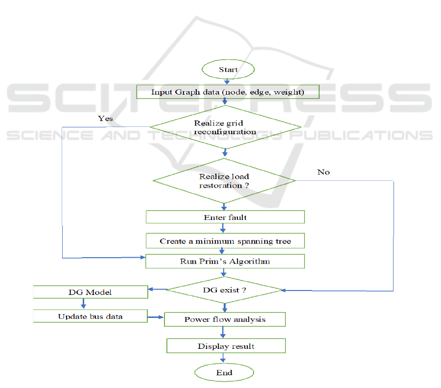
Figure 2: Flowchart of the proposed algorithm.

Restore Power Losses using the Hybrid of the Minimum Spanning Tree and Backward Forward Sweep

111

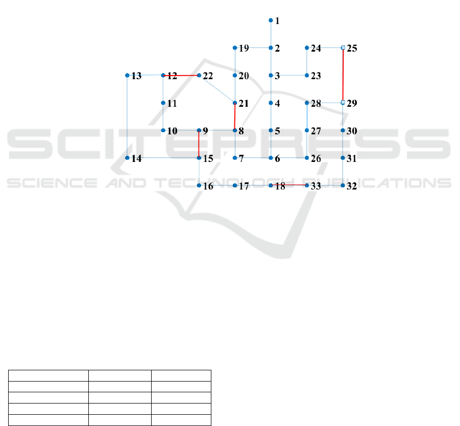
Figure 2 presents our suggested method to

minimize losses. To apply this method, we need to

have the line and load data of the network (impedance

of edges, active power, and reactive power of the

buses) also the location and size of the DG units.

Our proposed algorithm is focused on three main

steps:

Step 1: start by initializing the line and load data.

Step 2: create the minimum spanning tree by using

the prim’s algorithm (already described – figure 1)

Step 3: if DG units exist, update the load data of

the bus where DG is connected and apply load flow

analysis described in section 2.3.

Else Run load flow analysis until the algorithm

checks the constraints.

2.4.1 Networks without DGs

To check the reliability of our proposed algorithm, we

apply the electrical distribution network of 33 buses.

The electrical and topological features of this network

are taken from the reference of (Baran & Wu, 1989),

the table 4 in appendices shows the line data and load

data of the standard electrical network.

Figure 3 presents the reconfiguration of the

network of 33 buses before reconfiguration. With the

total reactive power equal 2.3 Mvar, the losses value

before reconfiguration equal 15.17% from the total

power, and the total active power equal 3.715 MW.

The network works at the nominal voltage 12.66 kV,

and the apparent base power is 100 MVA.

Figure 3: Network IEEE ‘’ 33 bus before reconfiguration’’.

This electrical system is constituted from 33

buses, and 37 edges, where we have 32 close edges,

and 5 open edges. As shown in figure 4, the red lines

are the set of the open switches.

2.4.2 Network with DGs

The second case is the network with the existence of

the DG units, in this paper, we assume that we have 4

DGs. Table 1 gives the data of the DG units injected.

Table 1: DGs data (Hossein Moarrefi, 2013).

Location

(

bus

)

Size

(

)

Power facto

28 0.1 0.95

17 0.2 0.95

2 0.14 0.98

32 0.25 0.85

As already described, the weight of the line, in this

case, is the resistance. So, the result before and after

the update of the line and load data is the same

because the injection of the DG has not any impact on

the resistance.

Otherwise, regarding the insertion of the DG

units, we must update the new active power and

reactive power of the node where the DG is injected,

then we apply the load flow analysis. For this reason,

we use the following equations 8, 9, and 10 (Seif,

2014).

P= P



- P



(8)

Q= Q



- Q



(9)



= a* Q



(10)

So, in this study, we consider the DG units as a

negative load, as shown in figure 4:

BML 2021 - INTERNATIONAL CONFERENCE ON BIG DATA, MODELLING AND MACHINE LEARNING (BML’21)

112

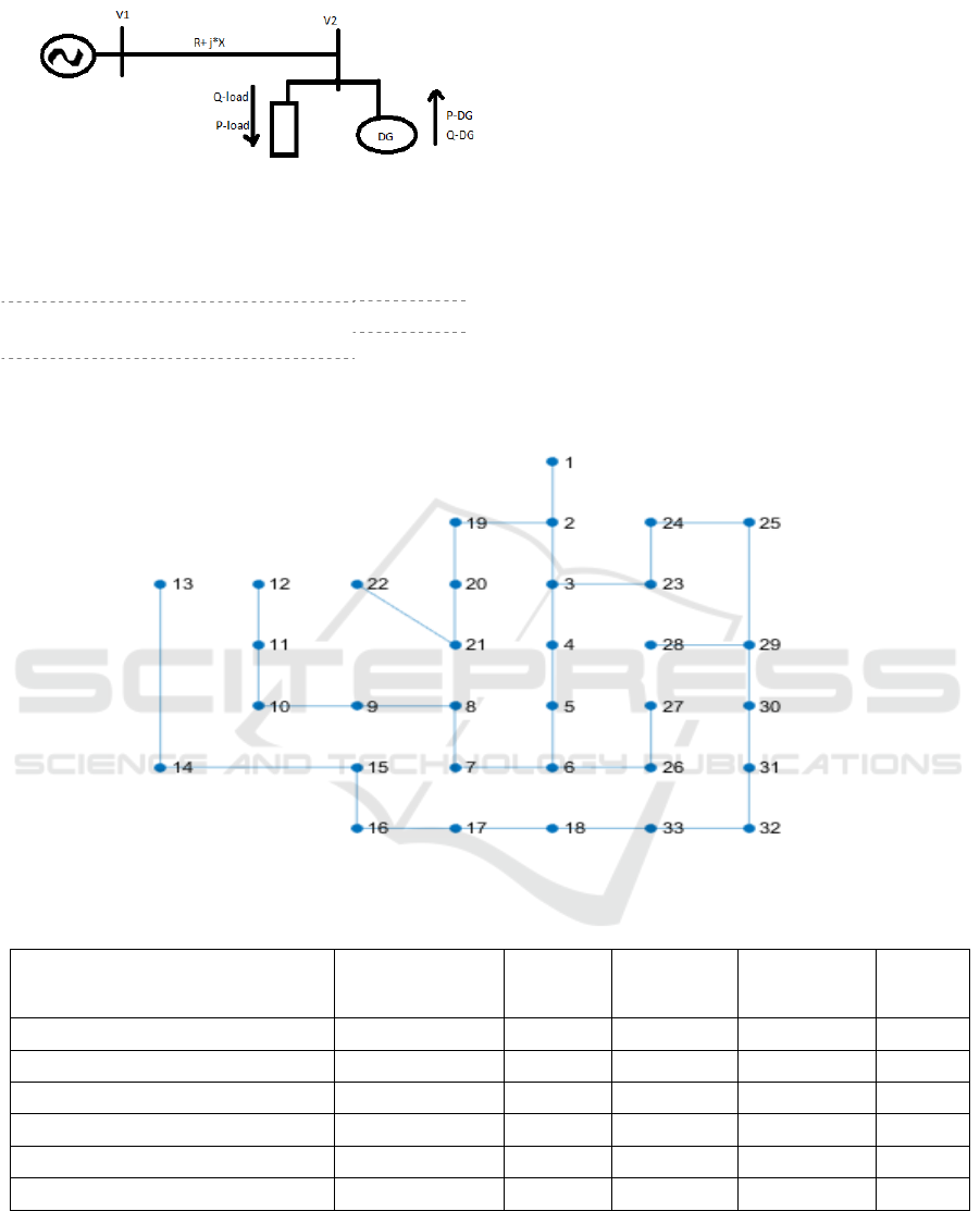
Figure 4: DG connected as a negative load to the bus.

After insertion of the DG unit, the new value of

the losses defined by equation 11:

𝑃



R∗



𝑃











+



𝑄



 𝑄







/𝑉



(11)

with:

R is the line resistance.

𝑃



presents the line losses.



is the active power consumption of the load.



is the reactive power consumption power.

P



, Q



) present the active and reactive power

output of distributed generation.

a: is the power factor of DG.

To check the performance of our proposed

algorithm, a comparative study is done.

3 TEST AND RESULTS

3.1 Case without DGs

Figure 5: Test system in MATLAB.

Table 2: Comparative analysis.

Tie line Power

losses Mw

Minimum

p.u.Voltage

Bus No of

minimum p.u.

volta

Time S

Base case 33- 34-35-36-37 0.2024 0.7717 33 -

Prim’s (proposed) 12-27-33-34-35 0.12489 0.95133 25 0.2235

Prim’s (TD s. , 2017) 7-8-13-29-37 0.1165 0.9446 30 -

Kruskal’s (Mohamad, 2019) 16-27-33-34-35 0.1786 0.9282 17 0.8566

BPSO & MSSO (JUMA S. A., 2018) 7-9-14-32-37 0.139 0.9479 18 34.63

Redefined Genetic 7-10-14-36-37 0.2007 0.8330 33 -

Restore Power Losses using the Hybrid of the Minimum Spanning Tree and Backward Forward Sweep

113

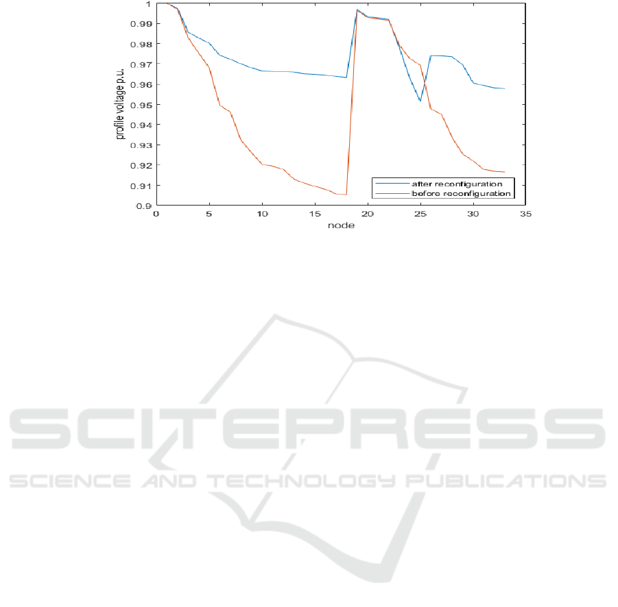
Figure 6: profile tension improvement.

After implementing of our line and load data, the new

reconfiguration is 12-27-33-34-35, as shown in figure

Table 2 presents the comparative study, and it is

noticed that when we use our proposed algorithm, the

losses are reduced and becomes 0.1248 Mw, instead

of 0.2024 MW for the standard case and 0.178 MW

for the case of new architecture using the Kruskal

algorithm, 0.139 MW for the BPSO algorithm, and

0.2007 MW for the case of reconfiguration by using

the redefined genetic algorithm.

Furthermore, table 2 indicates that the minimum

voltage of our proposed algorithm is 0.95133 p.u. at

node 18, this value respects the range limit of voltage.

Also, it is improved compared with the standard case

where the minimum voltage equal 0.7717 p.u. for the

Kruskal’s algorithm, the minimum voltage is 0.9282

p.u., for the BPSO it is noticed that the minimum

voltage is equal 0.9479p.u., and for the redefined

genetic, the minimum voltage is 0.8330p.u. So, we

conclude that our suggested method improves the

voltage profile better than the other recent studies.

Figure 6 and Table 2 present the performance of

the suggested prim’s algorithm compared with other

recent articles. The table in appendix B gives the

value found in each bus before and after the

restoration of active power loss by using the

reconfiguration of the network without DGs.

Finally, we conclude that our proposed algorithm

helps to minimize the active power loss and enhance

the voltage profile better than the other studies. Also,

this algorithm gives result in this case after 0.2235s,

this value it is lesser than the Kruskal's algorithm that

finds result after 0.8566s and lesser than the BPSO

algorithm that takes 34.64s. Appendix B gives the

voltage profile of each bus for the standard case and

our result.

3.2 Case with DGs

As presented previously, we consider that the weight

of edges is their resistance. Furthermore, the insertion

of the DG has not any impact on the impedance. So,

the implementation of the line data, in this case, gives

the same reconfiguration of the case of the network

without the presence of the DG after applying the

prim’s algorithm, as shown in figure 5. After this step,

we update the load data of the bus where the DG is

injected by using the equation (8), (9), and (10). Then

we apply the load flow method by using the main step

of the backward/ forward sweep (equation (5), (6),

and (7)).

Table 3 presents the simulation results of our

proposed algorithm in this case and the results of

other recent studies. Consequently, it is noted that the

losses found using our proposed algorithm equal

0.1331 MW; this value is big than the losses found by

(Hossein Moarrefi, 2013), where they have found

0.1241MW. However, it is important to note that the

losses of the standard case equal 0.2465 MW, and this

value is very big than our case.

Considering the voltage profile, our proposed

method enhances the voltage at each node better than

the base case and the (Hossein Moarrefi, 2013). Also,

the minimum voltage of our case equals 0.95025 p.u.

Nevertheless, in the case of the authors (Hossein

Moarrefi, 2013), the minimum voltage is 0.9124 p.u.

and 0.8950 p.u. for the base case. Furthermore, our

proposed algorithm gives the results after 0.2235 s.

Figure 7 presents the voltage profile curve in two

cases: the standard case and the case of our proposed

algorithm. It is noticed that the value of the voltage of

each node using our proposed algorithm is more

improved than the base case.

BML 2021 - INTERNATIONAL CONFERENCE ON BIG DATA, MODELLING AND MACHINE LEARNING (BML’21)

114

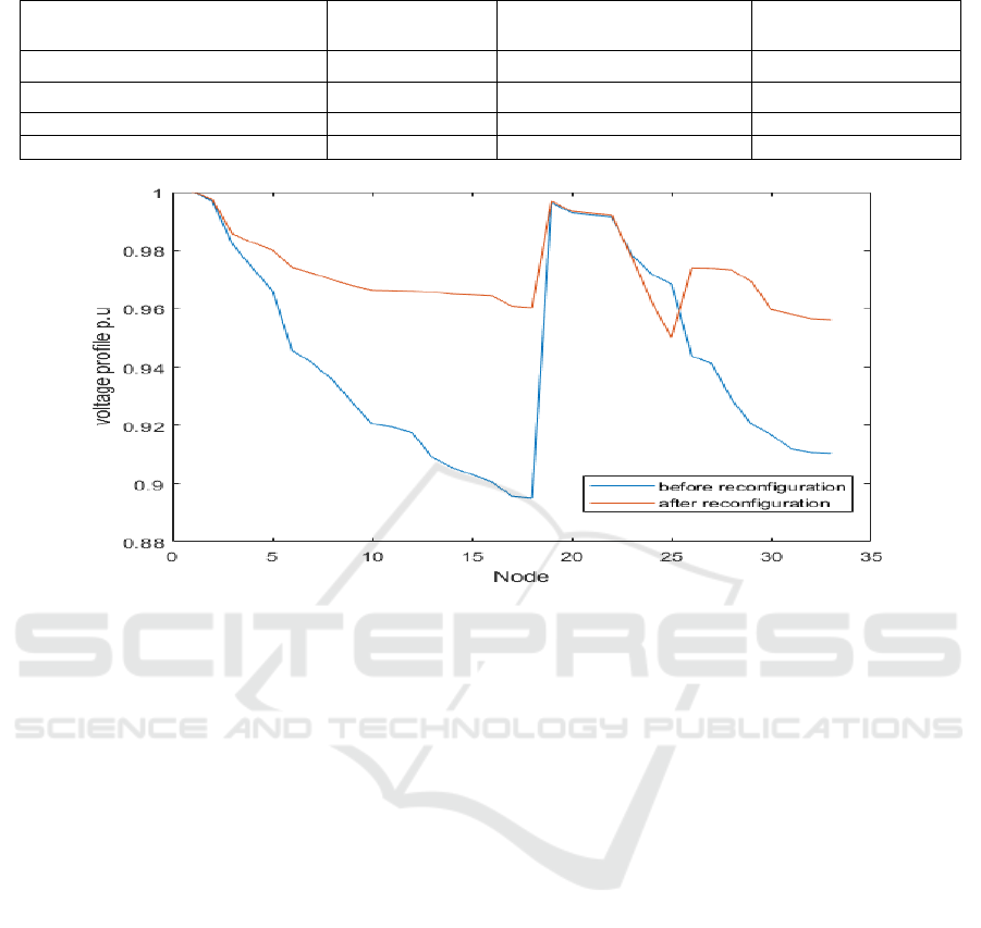
Table 3: Comparative analysis for case network with DG

Base case with

GA with DG (Hossein

Moarrefi, 2013)

Proposed prim’s

algorithm with DG

Open branches 33-34-35-36-37 12-15-18-21-22 12-27-33-34-35

The node of minimum voltage 18 - 25

Minimum voltage profile (p.u) 0.8950 0.9124 0.95025

Total losses (MW) 0.2465 0.1241 0.1331

Figure 7: voltage profile for radial system distribution with DGs.

So, considering the improvement of the voltage

profile, our study is perfect than the base case and the

study (Hossein Moarrefi, 2013). Table 5 presents the

value of the voltage before and after reconfiguration

using our method.

4 CONCLUSION

In this article, our objective is to restore the losses

aiming that the electrical plants can follow the

customer's request. So, for this reason, this study

proposes to use a combination of the prim’s algorithm

and the backward/ forward sweep due to their

advantages to find the minimum spanning tree and to

check the constraint with a higher speed to converge.

For the Prim’s algorithm, we have considered that the

weight of edges is the resistance of lines also is used

to check the constraint of the network have a radial

topology, for the backward/ forward sweep is used to

check the constraints of the current and voltage range

limit also the first law of Kirchhoff.

To check the quality and the reliability of our

study, we have used the electrical distribution

network of 33 buses for two cases: network without

and with the presence of the DG units. The simulation

results of these two cases show that our hybrid

method is perfect for minimizing losses and

enhancing the voltage at a lesser time compared with

other studies. For the next work, we advise using an

evolutionary algorithm to solve the problem aiming

to find the global optimum.

REFERENCES

Ahmad, S., Asar, A. U., Sardar, S., & Noor, B., 2017.

Impact of distributed generation on the reliability of

local distribution system. IJACSA International

Journal of Advanced Computer Science and

Applications, 8(6), 375-382.

Ahuja, A., & Pahwa, A., 2005. Using Aint Colony

Optimization for loss minimization in distribution

networks. Proceedings of the 37th Annual North

American Power Symposium, IEEE.

Alvarez-Hérault, & Marie-Cécile., 2010. Architectures des

réseaux de distribution du futur en présence de

production décentralisée, Sciences de l'ingénieur.

Grenoble: Institut National Pplythechnique de

Grenoble.

Baran, M. E., & Wu, F. F., 1989. Network reconfiguration

in distribution systems for loss reduction and load

balancing. IEEE Transactions on Power Delivery, 4(2),

1401 - 1407.

Restore Power Losses using the Hybrid of the Minimum Spanning Tree and Backward Forward Sweep

115

Caire, R., 2004. Gestion de la production décentralisée

dans les réseaux de distribution. tel-00007677: Institut

National Polytechnique de Grenoble.

Carreno, E. M., Romero, R., & Padilha-Feltrin, A., 2008.

An efcient codifcation to solve distribution network

reconfguration for loss reduction problem. IEEE

Transactions on Power Systems, 23(4), 1542-1551.

Chidanandappa, R., Ananthapadmanabha, T., & H.C., R.,

2015. Genetic algorithm based network reconfiguration

in distribution systems with Multiple DGs for time

varying loads. SMART GRID Technologies, 21, 460-

467.

Dodu, J., 1978. Modèle dynamique d’optimisation à long

terme d’un réseau de transport.

http://www.numdam.org/item?id=RO_1978__12_2_1

41_0.

Enacheanu, F. B., 2008. outils d’aide à la conduite pour les

opérateurs des réseaux. HAL https://tel.archives-

ouvertes.fr/tel-00245652.

Gallego, L. A., Carreno, E., & Padilha-Feltrin, A., 2010.

Distributed generation modeling for unbalanced three-

phase power flow calculations in smart grids.

Transmission and Distribution Conference and

Exposition: Latin America (T&D-LA).

Hasmaini, M., Zalnidzham, W. I., Salim, N. A., Shahbudin,

S., & Yasin, Z. M., 2019. Power system restoration in

distribution network using kruskal algorithm.

Indonesian Journal of Electrical Engineering and

Computer Science, 16(1), 8.

Hossein Moarrefi, M. N., 2013. Reconfiguration and

distributed Generation(DG) placement considering

critical system condition . 22nd International

Conference on Electricity Distribution . stockholm.

JUMA, S. A., 2018. Optimal radial distribution network

reconfiguration using modified shark smell

optimization. http://hdl.handle.net/123456789/4854.

Le Xie, & Marija D.Ilic., 2008. Model Predictive Dispatch

in Electric Energy Systems with Intermittent

Resources. IEEE International Conference on Systems,

Man and Cybernetics. IEEE.

Leonardo W. Oliveira, Edimar J. Oliveira, Ivo C. Silva,

Flávio V. Gomes, Thiago T. Borges, André L. M.

Marcato, & Ângelo R. Oliveira., 2015. Optimal

restoration of power distribution system through

particle swarm optimization. IEEE Eindhoven

PowerTech.

Ma, C., Li, C., Zhang, X., Li, G., & han, Y., 2017.

Reconfiguration of Distribution Networks with

Distributed Generation Using a Dual Hybrid Particle

Swarm Optimization Algorithm. Hindawi

Mathematical Problems in Engineering, 2017, 11.

Mohamad, H., 2019. Power system restoration in

distribution network using. Indonesian Journal of

Electrical Engineering and Computer Science, 16(1), 8.

Multon, B., 1999. L’énergie électrique: analyse des

resources et de la production. Journées de la section

électrotechnique du club EEA.

Ogunjuyigbe, A., Ayodele, T., & Akinola, O., 2016. Impact

of distributed generators on the power loss and voltage

profile of sub-transmission network. Journal of

Electrical Systems and Information Technology, 3, 94-

107.

Peng, F. Z., 2004. Editorial Special Issue on Distributed

Power Generation. IEEE TRANSACTIONS ON

POWER ELECTRONICS, 19(5), 2.

Saad Ouali, A. C., 2020. An Improved Backward/Forward

Sweep Power Flow Method Based on a New Network

Information Organization for Radial Distribution

Systems. Hindawi Journal of Electrical and Computer

Engineering, 2020(ID 5643410), 12.

Salama, M. M., & El-Khattam, W., 2004. Distributed

generation technologies,defnitions and benefts. Electric

Power Systems Research, 71(2), 119-128.

Seif, M. A., 2014. Optimal voltage control and loss

reduction in microgrid by active and reactive power

generation. Journal of Intelligent & Fuzzy Systems, 27,

1649–1658.

Sivkumar Mishra, Debapriya Das, & Subrata Paul., 2014.

A Simple Algorithm for Distribution System Load

Flow with Distributed Generation. IEEE International

Conference on Recent Advances and Innovations in

Engineering. Jaipur, India: IEEE International

Conference on Recent Advances and Innovations in

Engineering.

Strasser, T., Andrén, F., Kathan, J., Cecati, C., Buccella, C.,

Siano, P., Mařík, V., 2014. A Review of Architectures

and Concepts for Intelligence in Future Electric Energy

Systems,. IEEE Transactions on Industrial Electronics,

62(4), 2424 - 2438.

TD, s., 2017. loss minimization in distribution network by

using prim’s algorithm. International Journal of

Applied Engineering Research , 9(24), 15.

Tomoiaga, B., Chindris, M., Sumper, A., Villafafila-

Robles, R., & Sudria-Andreu, A., 2013. Distribution

system reconfiguration using genetic algorithm based

on connected graphs. Electric Power Systems Research

journal, 104(216-225), 10.

Zhongfu Jiang, Donglei Sun, Long Zhao, Xiaoming Li,

Shan Li, & Xueshan Han., 2017. A new method for

reference network considering network topology

optimization. 2017 Chinese Automation Congress

(CAC), IEEE.

BML 2021 - INTERNATIONAL CONFERENCE ON BIG DATA, MODELLING AND MACHINE LEARNING (BML’21)

116

APPENDIX

Table 4: line data and load data of IEEE 33 bus (Baran & Wu, 1989).

Line data Load data

Branch N° From bus To bus R (ohm) X(ohm) Pl(Kw) Ql(kvar)

1 1 2 0,0922 0,047 100 60

2 2 3 0,493 0,2511 90 40

3 3 4 0,366 0,1864 120 80

4 4 5 0,3811 0,1941 60 30

5 5 6 0,819 0,707 60 20

6 6 7 0,1872 0,6188 200 100

7 7 8 0,7114 0,2351 200 100

8 8 9 1,03 0,74 60 20

9 9 10 1,04 0,74 60 20

10 10 11 0,1966 0,065 45 30

11 11 12 0,3744 0,1238 60 35

12 12 13 1,468 1,155 60 35

13 13 14 0,5416 0,7129 120 80

14 14 15 0,591 0,526 60 10

15 15 16 0,7463 0,545 60 20

16 16 17 1,289 1,721 60 20

17 17 18 0,732 0,574 90 40

18 2 19 0,164 0,1565 90 40

19 19 20 1,5042 1,3554 90 40

20 20 21 0,4095 0,4784 90 40

21 21 22 0,7089 0,9373 90 40

22 3 23 0,4512 0,3083 90 50

23 23 24 0,898 0,7091 420 200

24 24 25 0,896 0,7011 420 200

25 6 26 0,203 0,1034 60 25

26 26 27 0,2842 0,1447 60 25

27 27 28 1,059 0,9337 60 20

28 28 29 0,8042 0,7006 120 70

29 29 30 0,5075 0,2585 200 600

30 30 31 0,9744 0,963 150 70

31 31 32 0,3105 0,3619 210 100

32 32 33 0,341 0,5302 60 40

Tie Lines

33 8 21 2 2

34 9 15 2 2

35 12 22 2 2

36 18 33 0,5 0,5

37 25 29 0,5 0,5

Restore Power Losses using the Hybrid of the Minimum Spanning Tree and Backward Forward Sweep

117

Table 5: Bus voltage before and after reconfiguration without DGs.

Network without DGs Network with DGs

Bus NO Voltage profile before

reconfiguration

Voltage profile after

reconfiguration

Voltage profile before

reconfiguration

Voltage profile after

reconfiguration

1 1 1 1 1

2 0.997 0.9975 0.9969 0.9975

3 0.9829 0.9857 0.9821 0.9856

4 0.9754 0.9828 0.9741 0.9827

5 0.968 0.9802 0.9662 0.9701

6 0.9496 0.9743 0.9458 0.9742

7 0.9461 0.9723 0.9413 0.9722

8 0.9324 0.9700 0.9357 0.9699

9 0.9261 0.9680 0.9279 0.9679

10 0.9203 0.9665 0.9205 0.9664

11 0.9194 0.9664 0.9194 0.9663

12 0.9176 0.9662 0.9176 0.9661

13 0.9131 0.9659 0.9091 0.9658

14 0.911 0.9651 0.9056 0.9650

15 0.9095 0.9648 0.9031 0.9647

16 0.908 0.9648 0.9007 0.9644

17 0.9058 0.9638 0.8957 0.9610

18 0.9052 0.9632 0.8951 0.9604

19 0.9965 0.9969 0.9964 0.9969

20 0.9929 0.9931 0.9928 0.9934

21 0.9922 0.9927 0..9921 0.9927

22 0.9916 0.9920 0.9915 0.9920

23 0.9793 0.9782 0.9785 0.9779

24 0.9727 0.9630 0.9718 0.9623

25 0.9693 0.9513 0.9685 0.9503

26 0.9477 0.9741 0.9438 0.9740

27 0.9451 0.9739 0.9412 0.9738

28 0.9337 0.9735 0.9290 0.9733

29 0.9255 0.9696 0.9204 0.9693

30 0.922 0.9606 0.9168 0.9597

31 0.9178 0.9596 0.9120 0.9581

32 0.9169 0.9582 0.9108 0.9566

33 0.9166 0.9579 0.9105 0.9563

BML 2021 - INTERNATIONAL CONFERENCE ON BIG DATA, MODELLING AND MACHINE LEARNING (BML’21)

118