Recurrent Neural Networks Analysis for Embedded Systems
Gonc¸alo Fontes Neves
a
, Jean-Baptiste Chaudron
b
and Arnaud Dion
c
ISAE-SUPAERO, Universit
´
e de Toulouse, France
Keywords:
Deep Learning, RNN, GRU, LSTM, Embedded Systems.
Abstract:
Artificial Neural Networks (ANNs) are biologically inspired algorithms especially efficient for pattern recog-
nition and data classification. In particular, Recurrent Neural Networks (RNN) are a specific type of ANNs
which model and process sequences of data that have temporal relationship. Thus, it introduces interesting
behavior for embedded systems applications such as autopilot systems. However, RNNs (and ANNs in gen-
eral) are computationally intensive algorithms, especially to allow the network to learn. This implies a wise
integration and proper analysis on the embedded systems that we gather these functionalities. We present
in this paper an analysis of two types of Recurrent Neural Networks, Long-Short Term Memory (LSTM)
and Gated-Recurrent Unit (GRU), explain their architectures and characteristics. We propose our dedicated
implementation which is tested and validated on embedded system devices with a dedicated dataset.
1 INTRODUCTION
As the industry and services change their business
models to be increasingly reliant on automation, the
search for ways to make machines more independent
and capable of interpreting the world by themselves
has rapidly increased. One way of doing this has
been through the many fields of the so called Artifi-
cial Intelligence (AI). The terms AI, Machine Learn-
ing (ML) and Deep Learning (DL) are often used in-
terchangeably, but must be seen as separate concepts
as they are, in fact, sub-fields of one another. Deep
Learning regroups various techniques and theories to
allow a digital processing unit to learn from a set of
data. Artificial Neural Networks (ANNs) are one of
the most used paradigm of Deep Learning which is
designed to mimic the principles and the behavior
of the neurons in a human brain. ANNs are able to
model a function by masking its complexity in a se-
ries of hidden layers which can be adjusted in size
and number. ANNs technology has grown exponen-
tially over the last years and is today at the heart of
scientific concerns for different applications in mul-
tiple research areas such as medicine with genome
analysis and general electronic health record track-
ing for predictive diagnosis (Yazhini and Loganathan,
2019), Natural Language Processing (NLP) (Kamis¸
a
https://orcid.org/0000-0001-6939-5096
b
https://orcid.org/0000-0002-2142-1336
c
https://orcid.org/0000-0002-1264-0879
and Goularas, 2019) or autopilot for self-driving ve-
hicles (Kulkarni et al., 2018)(Grigorescu et al., 2019).
In the context of the PRISE
1
project, we are in-
vestigating new concepts and techniques for embed-
ded systems such as next generation fault tolerant
flight control systems. As for cars autopilots (Grig-
orescu et al., 2019), we are interested in the integra-
tion of AI concepts for future Unmanned Aerial Vehi-
cle (UAV) and aircraft autopilots, such as learning the
pilot (or crew) skills and profile (Baomar and Bentley,
2016), or helping the pilot in difficult situations such
as landing with critical conditions (Baomar and Bent-
ley, 2017). Recurrent Neural Networks (RNNs) are a
specialized class of ANNs which can efficiently pro-
cess data that contains temporal relationships by inte-
grating a time dependent feedback loop in its memory.
This handling of temporal relation makes these types
of ANNs very promising for autopilot and flight con-
trol applications (Salehinejad et al., 2018)(Flores and
Flores, 2020). However, as embedded systems have
generally a limited amount of memory and process-
ing power (Rezk et al., 2020), the implementation of
RNNs must be carefully analysed.
This paper focuses on the study of two types of
RNNs: the Long-Short Term Memory (LSTM) and
the Gated-Recurrent Unit (GRU). We present here a
detailed analysis of their architectures and specifici-
ties. Then, we propose our own open-source imple-
1
French acronym for Platform for Embedded Systems
Research and Engineering
374
Neves, G., Chaudron, J. and Dion, A.
Recurrent Neural Networks Analysis for Embedded Systems.
DOI: 10.5220/0010715700003063
In Proceedings of the 13th International Joint Conference on Computational Intelligence (IJCCI 2021), pages 374-383
ISBN: 978-989-758-534-0; ISSN: 2184-3236
Copyright © 2023 by SCITEPRESS – Science and Technology Publications, Lda. Under CC license (CC BY-NC-ND 4.0)

mentation which has been validated on a dedicated
test case. This paper is organised as follow:
• Section 2 describes the state of the art for ANNs
and focuses on the specificities of RNNs.
• Section 3 explains how ANNs can learn with
back-propagation and what are the parameters to
consider for its implementation.
• Section 4 outlines the architectural aspects of
LSTM and GRU and their characteristics.
• Section 5 presents the experimentation details,
shows our results then section 6 concludes and of-
fers some perspectives for future work.
2 STATE OF THE ART
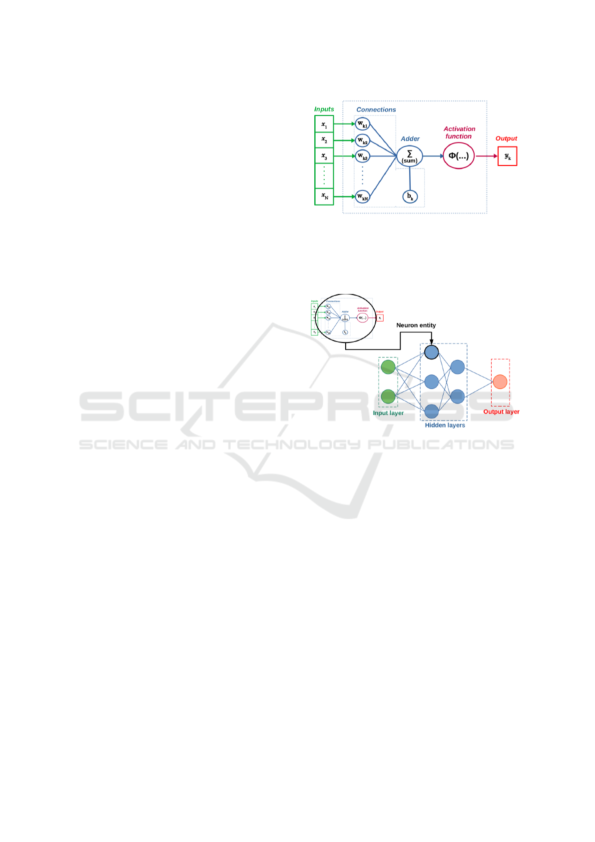
2.1 The Neuron Concept
A Neural Network, as defined by Haykin (Haykin,
1999), is a system made up of interconnections
between a large number of nonlinear processing
units called neurons. The first algorithm consid-
ered to implement a neuron was the perceptron algo-
rithm (Rosenblatt, 1957) which was trained as a bi-
nary classifier and immediately expanded to perform
the operations of logical gates such as the XOR gate.
From this baseline, new complex structures have been
developed but the basic building blocks of a neuron
remain usually fundamental to all types of structures
with three essential elements (Cf. Figure 1):
1. A set of connection, or synapses. Each connection
is associated with a weight (noted W
ki
in Figure 1).
This weight basically defines the influence of the
signal passing through the connection.
2. An adder function (
∑
in Figure 1) that sums the
weighted inputs of the neuron and the bias (addi-
tional parameter, noted b
k
).
3. An activation function (noted Φ(...) in Figure 1),
which is essentially the processing unit of the neu-
ron. The selection of this function is crucial in im-
plementation and the behavior of ANNs (see Sec-
tion 3.2).
2.2 Towards More Complex Structures
Moving on from the neuron basic building blocks of
the ANNs, the structure has been extended and up-
dated to create architectures with more neuron enti-
ties and layers, started with the three layers percep-
tron (Irie and Miyake, 1988). This introduced scala-
bility to the original model, with stacked neuron enti-
ties in an input layer, multiples hidden layers and an
Figure 1: Generic model of a neuron.
output layer such as depicted in Figure 2. These up-
dated structures allow new applications with the pos-
sibilities to model more complex systems and provide
more sophisticated outputs.
Figure 2: From neuron entity to MLP.
From this baseline, investigations have been per-
formed to extend these concepts to different problems
and applications. Nowadays, there are a lot of differ-
ent types of ANNs which can be combined and mixed.
However, the three majors types of ANNs remains:
• As explained previously, the Multi-Layer Percep-
tron MLP is an extended version of the original
perceptron (Irie and Miyake, 1988) that contains
three or more layers. Each layer has one or sev-
eral nodes (or neurons). Each node of a layer can
be fully or partially connected to the nodes of the
following layer.
• The Convolutional Neural Network CNN is a
variation of MLP that uses convolution operations
(matrix operations) between layers and shows out-
standing results in image classification and speech
recognition (Rawat and Wang, 2017).
• The Recurrent Neural Network RNN is analysed
in this paper and described in Section 2.3.
Recurrent Neural Networks Analysis for Embedded Systems
375

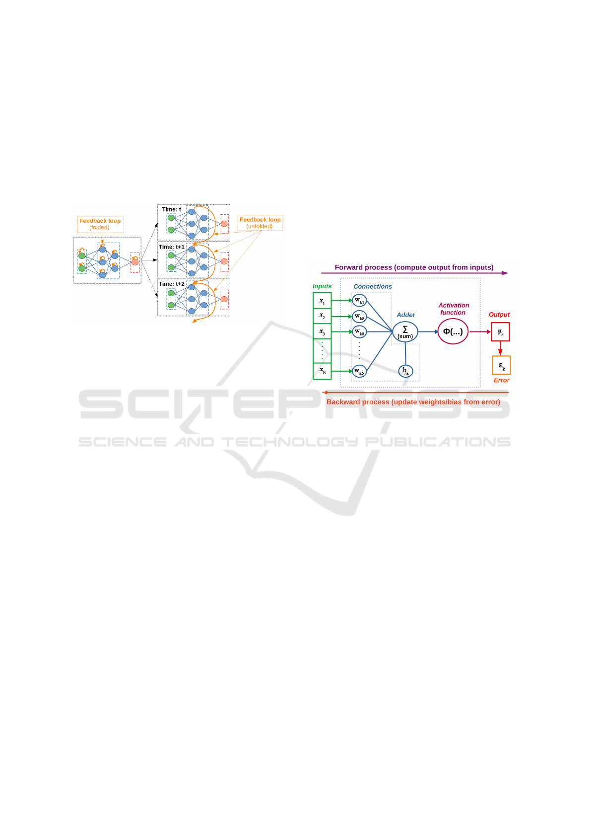
2.3 Recurrent Neural Networks (RNNs)
An RNN has an internal memory state creating a feed-
back loop. This principle allows a temporal relation-
ship between the data, the output of a cell is thus not
only influenced by the input but also by the previous
computations. Figure 3 shows this temporal relation-
ship from an folded RNN graph to an unfolded RNN
graph with the different time-steps.
Figure 3: Unfolding feedback loop for time relation.
The first version for RNNs was proposed in (El-
man, 1990) and was using this approach with feed-
back loop in the cells but it has shown a limitation.
When containing a large number of time steps and
cells, the RNNs were usually suffering from the van-
ishing gradient problem (Pascanu et al., 2013) during
training with back-propagation (explained in Section
3). Therefore, training such RNNs with any gradient-
based approach was difficult or even impossible due
to this exploding gradients phenomena (Rosindell and
Wong, 2018). Therefore, to tackle this issue, new spe-
cific RNNs architectures have been proposed. These
architectures overcome that by implementing sepa-
rate gates to add and, also, remove information about
past states. Nowadays, the two most popular RNNs
architectures are the LSTM (Gers et al., 2000) and
the GRU (Cho et al., 2014). As both outperform the
vanilla RNN (Chung et al., 2014), we have chosen
them for our work. They are described in Section 4.
3 BACK-PROPAGATION
3.1 Basic Principles
The heart of all ANN algorithms is the ability to learn
from experience. While the biological process is not
yet completely decoded, the attempts to mimic this
system have been studied for years. The first per-
ceptron model proposed by (Rosenblatt, 1957) had
some interesting concepts but had limited learning hy-
pothesis. Also, back in these days, the processing
machines were also not powerful enough to compute
large amount of data and to enable the capability of
learning (Minsky and Papert, 1969). The concept of
back-propagation was first introduced by Paul Werbos
in 1990 (Werbos, 1990). The main purpose of these
algorithms is to propagate the error signal generated
at the output per the feed-forward pass back across the
network. Thus, the contributions of each parameter
to the error can be calculated and used to correct the
weights of the connections and the biases. To sum up,
the feed-forward process generates the outputs from
the inputs and the back-propagation process updates
the weights and biases from the error in the opposite
direction (Cf. Figure 4).
Figure 4: Feed-forward and back-propagation illustration.
In large ANNs, this process happens layer by
layer, the error signal is first generated at the output
layer then propagated to each neuron. For RNNs, the
back-propagation, called Back-Propagation Through
Time (BPTT), consists of unfolding the whole neural
network (unrolling all the time-steps). Then, the error
is calculated from cell to cell, calculating the varia-
tions caused by the error from previous time-step us-
ing the chain rule to determine the derivative of each
operation from the feed-forward process. The goal
is to determine the error produced by the output with
respect to the temporal relationship (inherent to the
dataflow) and to calculate the corresponding gradi-
ents. These gradients are used to update the weights
and biases in order to decrease the error (see Section
3.3). To sum up, the back-propagation is based on two
concepts for all ANNs:
• A gradient calculation method which is based on
the first-order derivatives of the activation func-
tions φ(...) with respect to its input parameters.
• An optimization algorithm to update the weights
and bias from the gradient calculation.
NCTA 2021 - 13th International Conference on Neural Computation Theory and Applications
376

3.2 Activation Functions
The activation functions are functions that mimic the
behaviour of biological neurons. In the early days of
ANNs, the functions used were based on a threshold
logic output (basically ON or OFF). Then, the use of
nonlinear functions became essential to solve nontriv-
ial complex problems. For LSTM and GRU neural
networks, two activation functions are used, the sig-
moid and the hyperbolic tangent.
3.2.1 Sigmoid Activation Function
The sigmoid activation function, noted σ in this paper,
is a popular log based function that has been widely
used since the early days of ANNs. Equation 1 repre-
sents the function in exponential form. An interesting
characteristic of this function is that it maps all real
number to the range from 0 to 1.
σ(x) =
1
1 + e
−x
(1)
For back-propagation purpose, the gradient can be
expressed in terms of the function itself, as shown in
Equation 4. This is interesting for back-propagation
process because it allows less arithmetic operations.
σ
0
(x) = σ(x)(1 −σ(x)) (2)
3.2.2 Hyperbolic Tangent Activation Function
The hyperbolic tangent activation function, noted τ in
this paper, is another popular log based function. Sim-
ilar to the sigmoid function, the hyperbolic tangent
maps all real number between -1 and 1. The func-
tion can be expressed in exponential terms as shown
in Equation 3.
τ(x) = tanh(x) =
2
1 + e
−2x
−1 (3)
As the sigmoid function, for back-propagation
purpose, the gradient can be expressed in terms of the
function itself, as shown in Equation 4.
τ
0
(x) = 1 −τ(x)
2
(4)
3.3 Optimization Algorithms
The first choice made towards the back-propagation
algorithm is picking a loss function, meaning the
function that will provide the measurement for how
poorly the model is performing. For this work the
loss function used is the mean squared error (Brown-
lee, 2019) which is the average of the squared error
per output and per time-step. The expression (5) rep-
resents how this value is calculated where N is the
number of time-steps (in the time window under anal-
ysis) and M is the dimension of the output of the net-
work configuration.
Γ =
1
N
N
∑
i=1
(
1
M
M
∑
j=1
(λ
j
i
−y
j
i
)
2
) (5)
In our work, we have considered three optimiza-
tion algorithms, which are described in the follow-
ing sections. A survey of optimization algorithms for
back-propagation can be found in (Ruder, 2016). For
the sake of brevity of the notation, the parameters are
all referred to with θ and their gradients calculated
with ∇θ.
3.3.1 Stochastic Gradient Descent (SGD)
The SGD method with momentum (Qian, 1999) relies
on two hyper-parameters: the learning rate (noted α)
and the momentum (noted β). The tuning of the hyper
parameters was done maintaining the proposed value
for the momentum from (Ruder, 2016): β = 0.9. The
learning rate was trialled decrementally from 0.1 until
convergence was assured at α = 0.0001.
m
t
= (β −1)∇θ
t−1
+ β ·m
t−1
(6)
θ
t
= θ
t−1
−α ·m
t
(7)
3.3.2 Adam
The Adam method (Kingma and Ba, 2015) also re-
lies on learning rate and momentum (noted β
1
). It in-
troduces a second order term of momentum to calcu-
late the correction of the parameter as well as another
hyper-parameter (noted β
2
) to avoid division by zero
and assure numerical stability. The hyper-parameters
used for training with the Adam optimizer also fol-
lowed the proposed values from (Kingma and Ba,
2015): β
1
= 0.99 and β
2
= 0.999. The learning rate
was again decrementally tuned from 0.1 until conver-
gence was assured, this time at α = 0.001 and ε (addi-
tional parameter) was incrementally tuned from 10
−
8
until the oscillations in the testing learning curve were
achieved for ε = 10.0.
m
t
=
β
1
·m
t−1
+ (1 −β
1
) ·∇θ
t−1
1 −β
1
(8)
v
t
=
β
2
·v
t−1
+ (1 −β
2
) ·(∇θ
t−1
)
2
1 −β
2
(9)
θ
t
= θ
t−1
−
α ·m
t
√
v
t
+ ε
(10)
Recurrent Neural Networks Analysis for Embedded Systems
377

3.3.3 Adamax
Adamax is a variation of Adam, also proposed by
(Kingma and Ba, 2015), which uses exponentially
weighed norm instead of a second order momentum
term. The values of the hyper parameters used here
were the same as the ones used for Adam and pro-
duce the same desired convergence and stability.
u
t
= max(β
2
·u
t−1
, |∇θ
t−1
|) (11)
θ
t
= θ
t−1
−
α ·u
t
(1 −β
1
) ·ε
(12)
4 GRU/LSTM ARCHITECTURES
4.1 Notations
All the derivatives mentioned in this article are deriva-
tives of the output with respect to a certain vector or
matrix (Ξ):
∂Γ(e)
∂Φ
. However, for the sake of sim-
plicity, the derivatives will just be identified by what
they are with respect to: ∂Φ. This interpretation is to
be extended to the use of the ∇ symbol representing
gradients. This means that ∇Φ does not represent the
gradient of Φ but rather the gradient of the output with
respect to Φ.
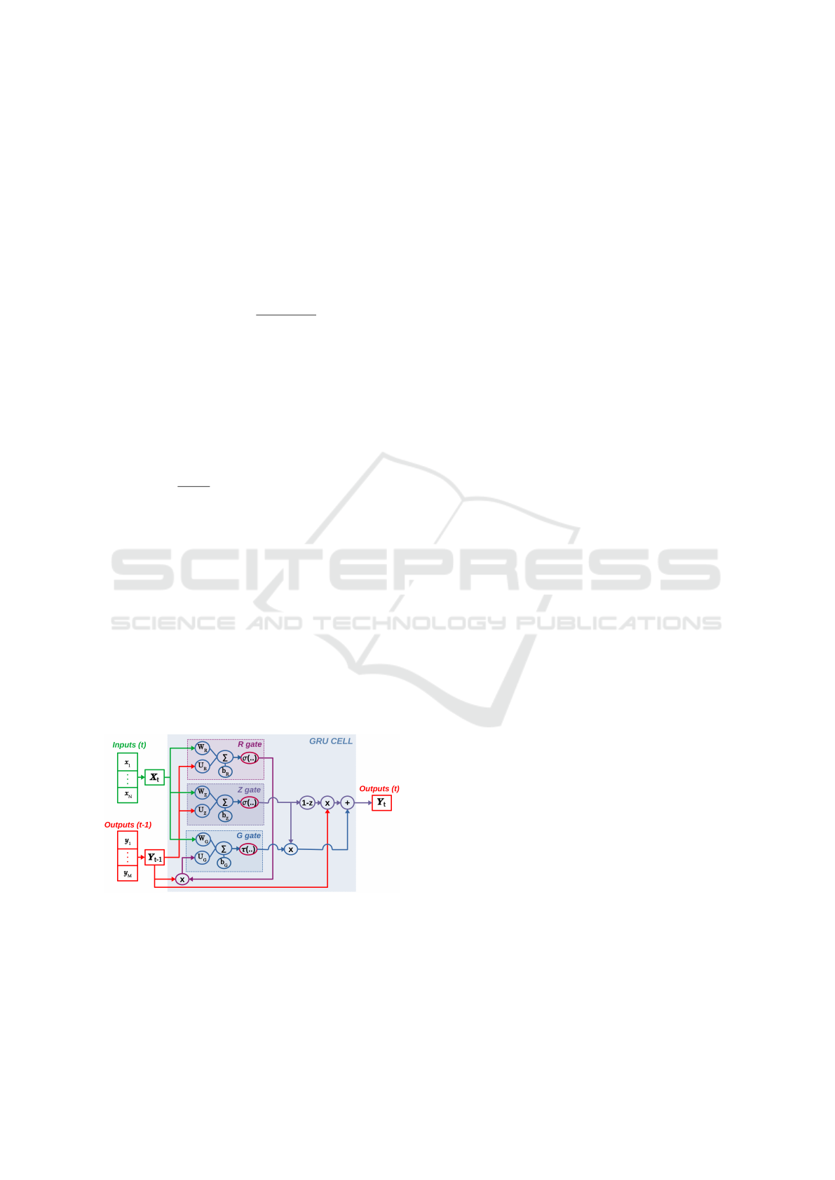
4.2 GRU Architecture
As can be seen in the schematic representation of the
GRU cell in Figure 5, the GRU architecture is com-
posed of three gates: the reset gate (R), the update
gate (Z) and the candidate gate (Z) (see expressions
(13), (14) and (15) for mathematical descriptions).
Figure 5: Anatomy of a GRU cell.
R
t
= σ(U
R
×Y
t−1
+W
R
×X
t
+ b
R
) (13)
Z
t
= σ(U
Z
×Y
t−1
+W
Z
×X
t
+ b
Z
) (14)
G
t
= τ(W
G
×X
t
+U
G
×(R
t
·Y
t−1
) + b
G
) (15)
The output for the step is calculated using the re-
sults of expression (16) where 1 represents a vector of
ones.
Y
t
= (1 −Z
t
) ·Y
t−1
+ Z
t
·G
t
(16)
These forward-propagation expressions and the
chain rule are used to determine the back-propagation
formulas. To recall, the goal is to establish the contri-
bution of the previous state vector to the error (as part
of BPTT) and the gradients of the weights and biases
of the current cell. Expressions (17), (18) and (19) are
the derivative of the output with respect to each gate.
This is then used to calculate each gate’s contribution
to the error of the model.
∂R
t
= σ
0
(R
t
) ·∂Y
t
·U
T
G
·∂G
t
(17)
∂Z
t
= σ
0
(Z
t
) ·∂Y
t
·(G
t
−Y
t−1
) (18)
∂G
t
= τ
0
(G
t
) ·∂Y
t
·Z
t
(19)
As stated, the expressions (20) and (21) are the
derivatives of the output with respect to the hidden
state and the input respectively, as part of unfolding
the network for BPTT.
∂Y
t−1
= U
T
R
×∂R
t
+U
T
Z
×∂Z
t
+ (U
T
G
·∂G
t
) ×R
t
+∂Y
t
×(1 −Z
t
)
(20)
∂X
t
= ∂R
t
×W
T
R
+ ∂Z
t
×W
T
Z
+ ∂G
t
×W
T
G
(21)
Expressions (22), (23) and (24) are the general
form to calculate the gradients in order to update
weights and bias with the back-propagation. The
expressions below abbreviate the gradients for all
weights and all biases where ξ ∈ {R, Z, G}.
∇W
ξ
= x
T
×∂ξ (22)
∇U
ξ
= h
T
×∂ξ (23)
∇b
ξ
= ∂ξ (24)
4.3 LSTM Architecture
LSTM cells store information about the stream of data
in two state vectors: a cell state (C
t
) which stores the
long-term memory of the cell and a hidden state (H
t
)
which handles the short-term memory and ultimately
renders the output of the cell at each instant. In this
paper, this hidden state (H
t
) is noted with its timing
representation depending on the output (Y
t−1
). The
activation of the state vectors is done by four gates:
the output gate (O), the candidate gate (G), the in-
put gate (I) and the forget gate (F). Expressions (25),
(26), (27) and (28) give the mathematical description
for these gates. The details about the LSTM cell struc-
ture are given in Figure 6. Note that some literature
NCTA 2021 - 13th International Conference on Neural Computation Theory and Applications
378

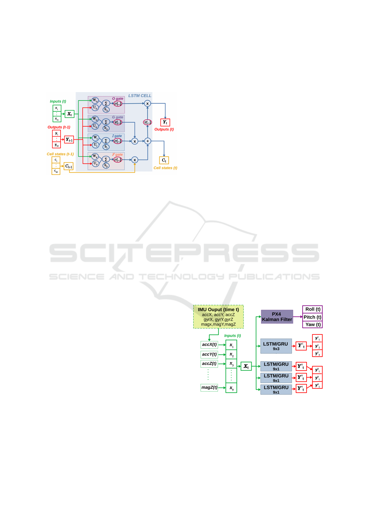
refers to the gates as layers because they perform a
similar transition as the one between layers of a MLP
network. However, in this paper, they will be referred
to as gates.
Figure 6: Anatomy of a LSTM cell.
O
t
= σ(X
t
×W
O
+Y
t−1
×U
O
+ b
O
) (25)
G
t
= τ(X
t
×W
G
+Y
t−1
×U
G
+ b
G
) (26)
I
t
= σ(X
t
×W
I
+Y
t−1
×U
I
+ b
I
) (27)
F
t
= σ(X
t
×W
F
+Y
t−1
×U
F
+ b
F
) (28)
The vectors that result from the computation of
the above expressions are directly used to determine
the following time-step of the hidden and cell states
according to (29) and (30).
C
t
= F
t
·C
t−1
+ I
t
·G
t
(29)
Y
t
= O
t
·C
t
(30)
Expressions (34), (33), (32) and (31) determine
the derivative of the output with respect to each gate.
This is then used to calculate each gate’s contribution
to the error of the model.
∂O
t
= σ
0
(O
t
) ·∂Y
t
·τ(C
t
) (31)
∂G
t
= τ
0
(G
t
) ·∂C
t
·I
t
(32)
∂I
t
= σ
0
(I
t
) ·∂C
t
·G
t
(33)
∂F
t
= σ
0
(F
t
) ·∂C
t
·C
t−1
(34)
Expressions (35), (36) and (37) determine one
of the mentioned goals of BPTT: the derivatives of
the output with respect to the previous cell state, the
previous hidden state and the input vector, respec-
tively. These calculations are used as input to the
back-propagation of the previous cell.
∂C
t−1
= ∂C
t−1
·F
t
+ ∂Y
t
·O
t
·τ
0
(C
t
) (35)
∂Y
t−1
= ∂G
t
×U
T
G
+ ∂I
t
×U
T
I
+ ∂F
t
×U
T
F
+∂O
t
×U
T
O
(36)
∂X
t
= ∂G
t
×W
T
G
+ ∂I
t
×W
T
I
+ ∂F
t
×W
T
F
+∂O
t
×W
T
O
(37)
The gradients for the update of the weights and the
bias can be calculated using the same expressions as
for the GRU (cf. Formulas (22), (23) and (24)) where
ξ ∈ {F, I, G, O}).
5 EXPERIMENTS AND RESULTS
5.1 Test Case Overview
To test our implementation, an Inertial Measure-
ment Unit (IMU) sensors fusion problem has been
taken. The values considered are the measurements
of the IMU containing accelerometers, gyroscopes,
and magnetometers as inputs and the roll, pitch and
yaw attitude angle as outputs. The reference out-
puts (called labels) have been given and sampled by
the PX4 autopilot using the dedicated (and calibrated)
Kalman filter (Garc
´
ıa et al., 2020). The data sets con-
tains 11 log files, each relative to a different flight of a
quad-copter UAV and generated with a sampling rate
of 100 Hz. Overall, each time step will use 9 inputs
(since each sensor produces measurements in x, y and
z axis) and up to 3 outputs for roll, pitch and yaw. We
have selected two types of LSTM/GRU structure, one
structure takes all the inputs to estimate all the outputs
(i.e. one single 9x3 structure) and the other is com-
posed of three LSTM/GRU structures that take all the
inputs to estimate each of the output separately (i.e.
three combined 9x1 structures). This is illustrated in
Figure 7. Note that the temporal window (number of
time-steps) for each structure is the same and equals
to 320 milliseconds (i.e. 32 time-steps at 100 Hz).
Figure 7: Test case illustration.
All log files loaded contributed with 70% of their
data to the training data set and 30% to the testing
data set. The batches included in each data set are not
contiguous, meaning that they were shuffled before
being divided into testing and training. The data-set
Recurrent Neural Networks Analysis for Embedded Systems
379

and our code are available as an open-source package
at: https://github.com/ISAE-PRISE/rnn4ap.
5.2 Data Normalization
The raw data from the IMU sensors are provided
in different units and oscillate within different in-
tervals and this introduce the problem of data scal-
ing (Brownlee, 2019). As described in subsection
3.2, the LSTM and GRU architectures are using the
sigmoid (σ) and the hyperbolic tangent (τ) as acti-
vation functions which provide outputs in [0, 1] and
[−1, 1] ranges respectively. Several options to scale
inputs for proper use of the activation functions were
studied (Sola and Sevilla, 1997). In our implemen-
tation, we have been using the scaling method which
combines a Z-score normalization with feature scal-
ing (Cf. Equation (38)) where µ is the average and σ
is the standard deviation.
y =
Z −min
max −min
with Z =
X −µ
σ
(38)
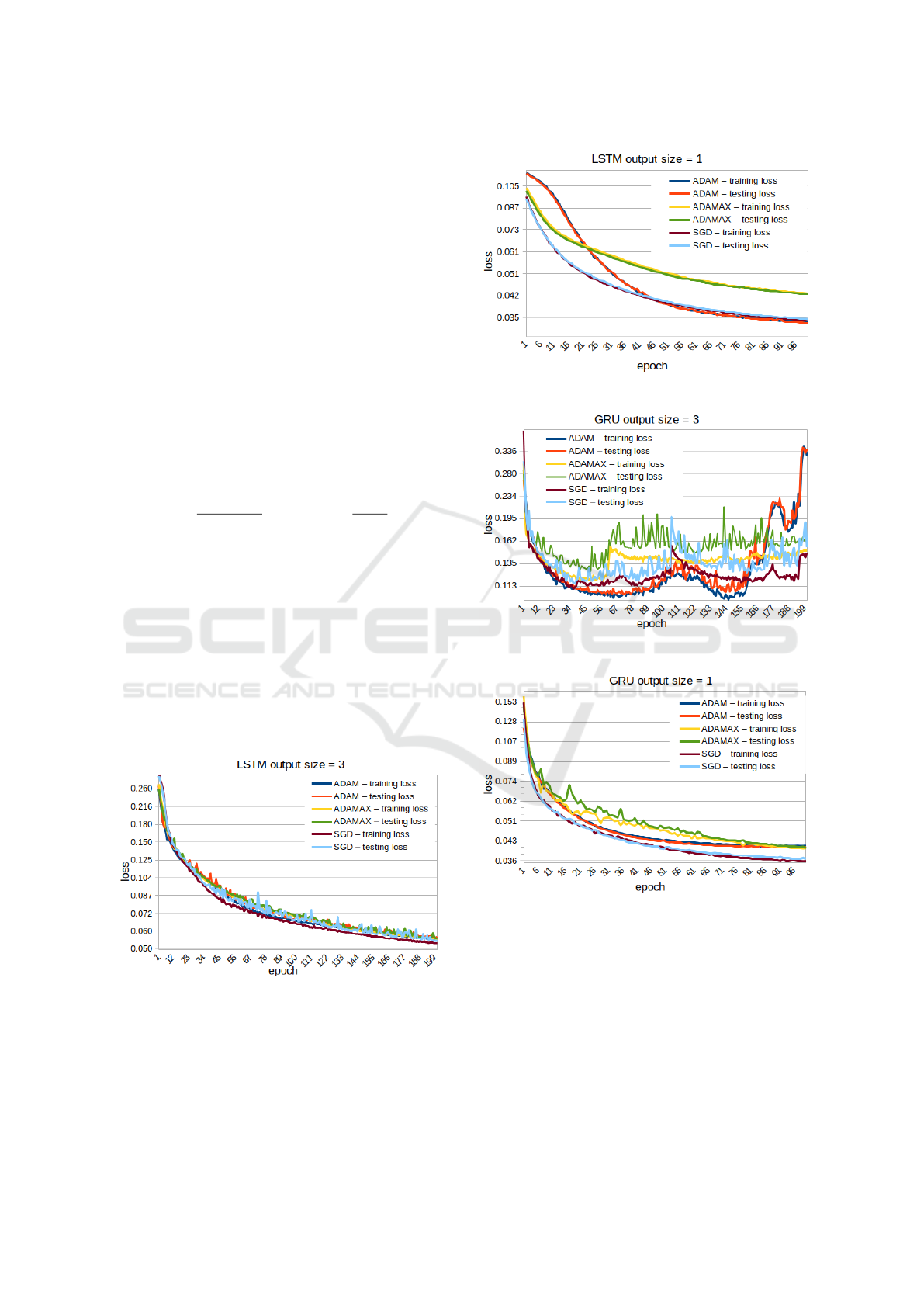
5.3 Training Results
The learning curves (evolution of training and testing
losses) are shown in Figures 9, 8, 11 and 10 for the
different configurations described in this paper. The
capability of a neural network to model a system in-
creases with its numerical complexity and the output
size. Thus, the 9x3 configurations took longer to train
and converge (around 200 epochs) while the 9x1 con-
figurations were only trained for 100 epochs to obtain
satisfying results.
Figure 8: Results of 200 epochs of training the LSTM 9x3.
The results of training the LSTM, in both config-
urations, present similar results for all optimizers ex-
cept for Adamax. It converges to a higher loss value
for the 9x1 configuration and presents for its train-
ing a slightly lower testing loss than training loss (this
Figure 9: Results of 100 epochs of training the LSTM 9x1.
Figure 10: Results of 200 epochs of training the GRU 9x3.
Figure 11: Results of 100 epochs of training the GRU 9x1.
could be a sign of under-fitting). For the GRU archi-
tectures, the 9x3 configuration behaves in an unpre-
dictable way after 60 epochs for all optimizers. This
means that after achieving a certain number of itera-
tions, the training process itself introduce error in the
model, making it impossible to be used. The 9x1 con-
figuration shows a better evolution even if Adamax
optimizer also suffers from issue seen for the LSTM.
Figure 12 shows the results (Targets versus Out-
puts) that are achieved with and 9x1 LSTM model
NCTA 2021 - 13th International Conference on Neural Computation Theory and Applications
380

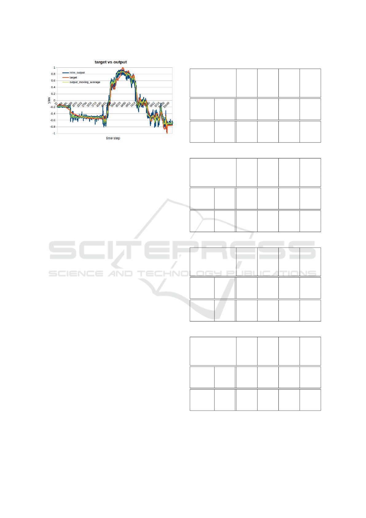
Figure 12: Targets vs Outputs for LSTM after training.
trained with SGD. Along with the output and the tar-
get a plot of the moving average of the output was
added to get a smoother version of the output, show-
ing that some operations to the output signal could
improve the final result.
5.4 Performance Results
Our GRU and LSTM prototypes have been imple-
mented in C++ using simple floating point precision
(i.e. 32 bits encoding) and have been tested on 4
embedded devices with different software configura-
tions:
1. Beaglebone AI with Linux Debian (kernel 4.14)
and gcc 6.3.0 (info: https://beagleboard.org/)
2. Raspberry 4 with Linux Raspy (kernel 5.10) and
gcc 8.3.0 (info: https://www.raspberrypi.org/)
3. Jetson Nano with Linux Ubuntu
(kernel 4.9) and gcc 7.5.0 (info:
https://developer.nvidia.com/embedded/)
4. Pynq Z2 with PetaLinux (kernel 4.19) and gcc
7.3.0 (info: http://www.pynq.io/)
The performance measurements obtained are pre-
sented in tables 1, 2, 3 and 4. The execution times
are expressed in milliseconds (ms) and represent the
duration of one execution step for a feed-forward
process (noted ff only) and one execution step for
a complete training process (feed-forward and back-
propagation, noted bp sgd). Note that all the training
algorithms implemented (see Section 3.3) have simi-
lar performance measurements therefore, for a sake of
clarity, we are only presenting the results from SGD.
6 CONCLUSION
This article focuses on the evaluation of RNNs for
real-time on-board applications. To do this, the the-
oretical background was analyzed in order to develop
Table 1: LSTM 9x3 performances on devices.
Boards bbai rpi4 pynq nano
(ms) (ms) (ms) (ms)
ff only
min 0.485 0.275 1.306 0.255
max 0.565 0.355 1.405 0.369
mean 0.491 0.294 1.316 0.259
bp sgd
min 2.619 1.720 7.390 1.680
max 3.147 1.927 7.651 1.958
mean 2.651 1.790 7.441 1.707
Table 2: LSTM 9x1 performances on devices.
Boards bbai rpi4 pynq nano
(ms) (ms) (ms) (ms)
ff only
min 0.185 0.102 0.476 0.091
max 0.225 0.145 0.544 0.142
mean 0.187 0.108 0.480 0.094
bp sgd
min 0.826 0.501 2.255 0.489
max 0.937 0.660 2.334 0.582
mean 0.835 0.536 2.27 0.497
Table 3: GRU 9x3 performances on devices.
Boards bbai rpi4 pynq nano
(ms) (ms) (ms) (ms)
ff only
min 0.370 0.212 1.022 0.190
max 0.418 0.276 1.066 0.268
mean 0.374 0.227 1.029 0.193
bp sgd
min 1.990 1.290 5.602 1.222
max 2.482 1.452 5.950 1.414
mean 2.013 1.340 5.639 1.242
Table 4: GRU 9x1 performances on devices.
Boards bbai rpi4 pynq nano
(ms) (ms) (ms) (ms)
ff only
min 0.145 0.081 0.382 0.070
max 0.174 0.132 0.417 0.102
mean 0.148 0.085 0.386 0.072
bp sgd
min 0.633 0.384 1.741 0.368
max 1.132 0.480 1.845 0.440
mean 0.643 0.410 1.756 0.372
our own optimal implementation of LSTM and GRU.
The analysis compared several configurations differ-
ing in algebraic complexity and optimization algo-
rithms. Finally, our implementation was success-
Recurrent Neural Networks Analysis for Embedded Systems
381

fully tested on various embedded targets with lim-
ited computing capacity and latency, showing that a
pre-trained LSTM or GRU can be embedded on such
devices (for example to complement a Kalman Fil-
ter for fault-tolerance purposes). However, the train-
ing phase is still too greedy in term of computing re-
sources to allow an online training capacity for em-
bedded devices. One benefit of our work is the release
of an open-source package including source code,
data-sets and logs. Therefore, our application with
its implementation details (and the results) are acces-
sible, can be used, reproduced and extended.
Two important future investigations would be to
migrate our implementation to a GPU based version
(using the GPU entity of the Jetson Nano device for
example) and also to create a FPGA based architec-
ture (using the FPGA entity of the Pynq Z2 device for
example). This would enables (1) the possibility to
run large LSTM/GRU neural networks and (2) tackle
online training capacities which can be key for em-
bedded systems algorithms dealing with uncertainties
in their environment. Our first efforts regarding GPU
and FPGA based architectures are very encouraging.
From the LSTM/GRU architecture point of view, we
are currently exploring the possibility of modeling the
autopilot data using a bi-directional configuration for
GRU and LSTM such as it has been done for ma-
chine translation applications (Schuster and Paliwal,
1997) (Sutskever et al., 2014). Last but not least,
even if the results obtained for the proposed test case
were sufficient to make the desired analysis, it has to
be extended. A real life application using RNNs re-
quires more effort for the training part especially on
the training dataset, therefore we are working now on
building a more dense dataset (for example to include
a lot more flight conditions or UAV types).
ACKNOWLEDGEMENTS
This work has been partially supported by
the Defense Innovation Agency (AID) of the
French Ministry of Defense under Grant No.:
2018.60.0072.00.470.75.01.
REFERENCES
Baomar, H. and Bentley, P. (2017). Autonomous landing
and go-around of airliners under severe weather con-
ditions using artificial neural networks. 2017 Work-
shop on Research, Education and Development of Un-
manned Aerial Systems (RED-UAS), pages 162–167.
Baomar, H. and Bentley, P. J. (2016). An intelligent au-
topilot system that learns piloting skills from human
pilots by imitation. In 2016 International Conference
on Unmanned Aircraft Systems (ICUAS), pages 1023–
1031.
Brownlee, J. (2019). Loss and Loss Functions for Training
Deep Learning Neural Networks.
Cho, K., Van Merri
¨
enboer, B., Gulcehre, C., Bahdanau, D.,
Bougares, F., Schwenk, H., and Bengio, Y. (2014).
Learning phrase representations using RNN encoder-
decoder for statistical machine translation. EMNLP
2014 - 2014 Conference on Empirical Methods in Nat-
ural Language Processing, Proceedings of the Confer-
ence, pages 1724–1734.
Chung, J., Gulcehre, C., Cho, K., and Bengio, Y. (2014).
Empirical Evaluation of Gated Recurrent Neural Net-
works on Sequence Modeling. pages 1–9.
Elman, J. L. (1990). Finding structure in time. Cognitive
Science, 14(2):179–211.
Flores, A. and Flores, G. (2020). Transition control of a
tail-sitter uav using recurrent neural networks. In 2020
International Conference on Unmanned Aircraft Sys-
tems (ICUAS), pages 303–309.
Garc
´
ıa, J., Molina, J. M., and Trincado, J. (2020). Real eval-
uation for designing sensor fusion in uav platforms.
Information Fusion, 63:136–152.
Gers, F. A., Schmidhuber, J. A., and Cummins, F. A. (2000).
Learning to forget: Continual prediction with lstm.
Neural Comput., 12(10):2451–2471.
Grigorescu, S. M., Trasnea, B., Cocias, T. T., and Mace-
sanu, G. (2019). A survey of deep learning techniques
for autonomous driving. CoRR, abs/1910.07738.
Haykin, S. (1999). Neural Networks: A Comprehensive
Foundation. Prentice Hall, Upper Saddle River, NJ.
2nd edition.
Irie and Miyake (1988). Capabilities of three-layered per-
ceptrons. In IEEE 1988 International Conference on
Neural Networks, pages 641–648 vol.1.
Kamis¸, S. and Goularas, D. (2019). Evaluation of Deep
Learning Techniques in Sentiment Analysis from
Twitter Data. Proceedings - 2019 International Con-
ference on Deep Learning and Machine Learning in
Emerging Applications, Deep-ML 2019, pages 12–17.
Kingma, D. P. and Ba, J. (2015). Adam: A method for
stochastic optimization. In Bengio, Y. and LeCun,
Y., editors, 3rd International Conference on Learn-
ing Representations, ICLR 2015, San Diego, CA, USA,
May 7-9, 2015, Conference Track Proceedings.
Kulkarni, R., Dhavalikar, S., and Bangar, S. (2018). Traffic
Light Detection and Recognition for Self Driving Cars
Using Deep Learning. Proceedings - 2018 4th Inter-
national Conference on Computing, Communication
Control and Automation, ICCUBEA 2018, pages 2–5.
Minsky, M. and Papert, S. A. (1969). Perceptrons: An Intro-
duction to Computational Geometry. The MIT Press.
Pascanu, R., Mikolov, T., and Bengio, Y. (2013). On
the difficulty of training recurrent neural networks.
In Proceedings of the 30th International Confer-
ence on International Conference on Machine Learn-
ing - Volume 28, ICML’13, page III–1310–III–1318.
JMLR.org.
NCTA 2021 - 13th International Conference on Neural Computation Theory and Applications
382

Qian, N. (1999). On the momentum term in gradi-
ent descent learning algorithms. Neural Networks,
12(1):145–151.
Rawat, W. and Wang, Z. (2017). Deep Convolutional Neu-
ral Networks for Image Classification: A Comprehen-
sive Review. Neural Computation, 29(9):2352–2449.
Rezk, N. M., Purnaprajna, M., Nordstrom, T., and Ul-
Abdin, Z. (2020). Recurrent neural networks: An
embedded computing perspective. IEEE Access,
8:57967–57996.
Rosenblatt, F. (1957). The Perceptron - A Perceiving and
Recognizing Automaton. Technical Report 85-460-1,
Cornell Aeronautical Laboratory.
Rosindell, J. and Wong, Y. (2018). Biodiversity, the tree
of life, and science communication. Phylogenetic Di-
versity: Applications and Challenges in Biodiversity
Science, (2):41–71.
Ruder, S. (2016). An overview of gradient descent opti-
mization algorithms. CoRR, abs/1609.04747.
Salehinejad, H., Baarbe, J., Sankar, S., Barfett, J., Colak, E.,
and Valaee, S. (2018). Recent advances in recurrent
neural networks. CoRR, abs/1801.01078.
Schuster, M. and Paliwal, K. (1997). Bidirectional recur-
rent neural networks. IEEE Transactions on Signal
Processing, 45:2673 – 2681.
Sola, J. and Sevilla, J. (1997). Importance of input data
normalization for the application of neural networks
to complex industrial problems. IEEE Transactions
on Nuclear Science, 44(3 PART 3):1464–1468.
Sutskever, I., Vinyals, O., and Le, Q. V. (2014). Sequence
to sequence learning with neural networks. CoRR,
abs/1409.3215.
Werbos, P. J. (1990). Backpropagation Through Time:
What It Does and How to Do It. Proceedings of the
IEEE, 78(10):1550–1560.
Yazhini, K. and Loganathan, D. (2019). A state of art ap-
proaches on deep learning models in healthcare: An
application perspective. Proceedings of the Interna-
tional Conference on Trends in Electronics and Infor-
matics, ICOEI 2019, (Icoei):195–200.
Recurrent Neural Networks Analysis for Embedded Systems
383