
Subset Sum and the Distribution of Information
Daan Van Den Berg
1 a
and Pieter Adriaans
2 b
1
Yamasan Science & Education, Amsterdam, The Netherlands
2
ILLC, IVI-CCI, University of Amsterdam, The Netherlands
Keywords:
Subset Sum, Branch and Bound, Information, Instance Hardness, Computational Complexity, NP-hard.
Abstract:
The complexity of the subset sum problem does not only depend on the lack of an exact algorithm that runs
in subexponential time with the number of input values. It also critically depends on the number of bits m of
the typical integer in the input: a subset sum instance of n with large m has fewer solutions than a subset sum
instance with relatively small m.
Empirical evidence from this study suggests that this image of complexity has a more fine-grained structure. A
depth-first branch and bound algorithm deployed to the integer partition problem (a special case of subset sum)
shows that for this experiment, its hardest instances reside in a region where informational bits are equally dis-
persed among the integers. Its easiest instances reside there too, but in regions of more eccentric informational
dispersion, hardness is much less volatile among instances. The boundary between these hardness regions is
given by instances in which the i
th
element is an integer of exactly i bits. These findings show that, for this
experiment, a very clear hardness classification can be made even on the basis of information dispersal, even
for subset sum instances with identical values of n and m. The role of the ‘scale free’ region are discussed
from an information theoretical perspective.
1 INTRODUCTION
The subset sum problem exists in many shapes
and forms, but always involves a set of integers
S = {x
1
, x
2
...x
i
...x
n
}, a target value t, and a summing
operation. Consider the following instance with
n = 8:
S = {1, 4, 9, 12, 17, 31, 41, 59} with t = 74
In its decision form (“Is there a subset of S that sums
up to t?”), the problem is in NP, because any given
solution can be verified for correctness in polyno-
mial time (Garey and Johnson, 1979). The subset
{41, 31, 1} is not a solution, because it sums up to 73
and not 74. Neither is {59, 9, 4, 1} and again, verify-
ing that it isn’t can be done quickly, by just summing
up the elements which takes polynomial time. Does
the above example have an exact solution at all?
Avoiding the direct answer to that question leads
to the slightly harder optimization problem (“Which
summed subset of S approximates t most closely?”).
This version of subset sum is NP-hard, and does not
a
https://orcid.org/0000-0001-5060-3342
b
https://orcid.org/0000-0002-8473-7856
have a polynomial time verification procedure. Sub-
set {41, 31, 1} might be the closest approximation, but
there’s no way of knowing for sure apart from sum-
ming all subsets of S, which is a cumbersome (non-
polynomial) operation.
This study focuses on the optimization problem,
with the additional requirement that t has the value
of the summed integers divided by two (which would
mean t = 87 in the above example). This version
is known as the partition problem
1
, and traditionally
formulated as the task to split the set into two as-
equal-as-possible valued subsets. In this paper, we’ll
use an exact algorithm, guaranteed to deliver the best
possible answer, and measure runtimes to assess the
hardness of individual problem instances.
There is some previous work related to ours. Early
papers by Brickell (Brickell, 1984) and Lagarias and
Odlyzko (Lagarias and Odlyzko, 1985) define den-
sity on knapsack and subset sum instances, and a
more recent work by Tural on the closely related de-
cision variant of subset sum also incorporates branch
and bound (Kemal Tural, 2020). His generation of
instances appears to be somewhat similar to that of
Zhang and Korf’s (Zhang and Korf, 1996), and al-
1
Or sometimes number partition problem
134
Van Den Berg, D. and Adriaans, P.
Subset Sum and the Distribution of Information.
DOI: 10.5220/0010673200003063
In Proceedings of the 13th International Joint Conference on Computational Intelligence (IJCCI 2021), pages 134-140
ISBN: 978-989-758-534-0; ISSN: 2184-3236
Copyright © 2023 by SCITEPRESS – Science and Technology Publications, Lda. Under CC license (CC BY-NC-ND 4.0)

though that study is on ATSP, we feel that our current
work is most supplementary to theirs. We’ll elaborate
a little more on this in Section 6.
The major difference with previous studies lies in
the creation of instances. Historically, this is often
done uniformly random from a range of integers. In
this study, we’ll take a different approach. All in-
stances in our experiment will have exactly 12 ele-
ments, exactly 78 bits of information, and are there-
fore supposedly equally hard. But by assigning an
explicit distribution to the informational bits of the el-
ements x
i
∈ S in an instance, we will show that this
distribution can also play a key role in the hardness
assessment of problem instances. The results of this
new approach makes us rethink the traditional hard-
ness measures, maybe even classes, and opens up a
whole new dimension of research in algorithms and
instance hardness. There’s also an information the-
oretical perspective on the results, which we’ll high-
light in Section 4.
2 METHODS
2.1 Branch & Bound
The solving algorithm for this experiment is rela-
tively straightforward. The term ‘branch and bound’
was coined by Little et al. (Little et al., 1963)(Daan
van den Berg, 2019)
2
but the basic principle ex-
isted earlier (Rossman and Twery, 1958a)(Rossman
and Twery, 1958b)(Eastman, 1958)
3
(Land and Doig,
2010)(Land and Doig, 1960)
4
. The paradigm appears
in roughly two algorithmic forms: a (priority) queue
based implementation and a stack-based implementa-
tion, which thereby follows a depth-first search tree
traversal. We will use the latter of the two, but both
forms are exact methods, and therefore guarantee a
solution iff it exists for any decision problem it is
deployed to, or return a 100% certain “no solution”
otherwise – given it has enough runtime to finish.
Along the same lines, depth-first branch and bound
is also solution-optimal when deployed to optimiza-
tion problems, guaranteeing the best solution when
it finishes. The drawback of course, is that runtimes
2
Little et al.’s original published paper is digitally avail-
able only as a murky scan, or a work-in-progress-report, but
the second reference points towards a fully refurbished edi-
tion, clean and searchable, made available in 2020.
3
Most of these works are very old, outdating the inter-
net, and not readily available in digital form.
4
Although both references point to the same paper, the
second one seems to be a republication. The original paper
is from 1960.
go up exponentially, exceeding the universe’s lifes-
pan even for moderately sized problem instances. Our
implementation on the subset sum problem has com-
plexity O(2
n
), but it does have a strong strategy for
cutting down runtimes. Abiding by Steven Skiena’s
famous words “Clever pruning can make short work
of surprisingly hard problems” (Skiena, 1998), it cuts
branches from the search tree which are guaranteed to
not improve over the incumbent best solution (‘best’).
For subset sum, this means that when the algorithm is
approximating t, and has a current value cur higher
that t, no additional items are added to it, using t as a
bound when branching through the search space. The
algorithm thus effectively traverses all 2
|S|
sums, but
omits branches that cannot possibly result in a better
value than the incumbent best, thereby saving signif-
icant computation time. Finally, the boolean variable
targetFound ensures the algorithm halts as soon as
the first exact solution is found.
1. Preprocessing: sort S in descending order, as-
sign cur := 0, i := 1, i
max
:= |S|,best := ∞, t =
1
2
∑
|S|
i=1
x
i
, targetFound := f alse.
2. Assign cur
1
:= cur + s
i
, cur
2
:= cur. If cur
1
= t,
then assign targetFound := true. If cur
1
< best :
best := cur
1
.
3. If i < i
max
and cur
1
< t and ¬targetFound: go to
2 with cur := cur
1
, i = i + 1.
4. If i < i
max
and cur
2
< t and ¬targetFound: go to
2 with cur := cur
2
, i = i + 1.
The reason that t is chosen for the bound, and not best,
is that in general, the closest possible approximation
can be either higher or lower than t. So if at some
point in the previous example cur = 68, the incum-
bent best solution best = 71 and t = 74, it is unwise
to cut off along best, because 75 is still achievable,
be it on the other side of t. Only when cutting off
after the last addition has exceeded t assures further
addition cannot result in a better solution.
2.2 Templates & Instances
We fed the solving algorithm exactly 70 instances di-
vided in 7 cohorts of 10 instances, each of which had
m = 78 bits of information in n = 12 positive integers
in its set. Every cohort was formed through a ‘strict
template’ that assigned a prespecified number of bits
b to every integer in the instance. As such, a 3-bit
template entry (‘3b’) results in a random integer, val-
ued 4, 5, 6 or 7 in the instance. The template entry 6b
results in an randomly chosen integer between 32 and
64 in the problem instance (some explicit examples
are in Table 1). It is important to observe the notion
Subset Sum and the Distribution of Information
135

Table 1: Seven ‘strict templates’ used for making 70 subset sum instances. A value such as 4b randomly generates a corre-
sponding integer of exactly 4 bits, meaning it is randomly chosen between 8 and 16. The templates vary in eccentricity, ST
3
being the most eccentric, and ST
−3
being the flattest possible. For each template, one corresponding instance is given as an
example.
Strict Template Example Instance
ST
3
(1b,1b,1b,1b,1b,4b,4b,5b,9b,13b,17b,21b) {0,1,1,1,0,10,12,17,478,7899,90607,1638220}
ST
2
(1b,1b,2b,2b,3b,4b,5b,6b,9b,12b,15b,18b) {1,1,3,3,6,15,23,40,423,3422,24181,251636}
ST
1
(1b,1b,2b,4b,4b,5b,6b,7b,9b,11b,13b,15b) {0,1,3,8,14,30,45,79,324,1145,4332,19120}
ST
0
(1b,2b,3b,4b,5b,6b,7b,8b,9b,10b,11b,12b) {1,2,6,12,19,35,115,247,305,563,1534,3828}
ST
−1
(3b,3b,4b,4b,5b,6b,7b,8b,8b,9b,10b,11b) {7,6,9,13,16,55,109,175,230,330,909,1686}
ST
−2
(4b,4b,5b,5b,6b,6b,7b,7b,8b,8b,9b,9b) {11,11,30,26,49,49,84,80,166,156,484,317}
ST
−3
(6b,6b,6b,6b,6b,6b,7b,7b,7b,7b,7b,7b) {58,54,35,61,50,49,122,71,111,119,108,92}
of ‘strict’, which means that a template entry of 6b
results in an integer of exactly 6 bits, and not fewer.
This constraint ensures that all instances in all cohorts
have exactly 78 bits in total, making all experimen-
tal instances equal in both n and m. Still, despite this
stringent uniformity, the exact assignment of informa-
tional bits within the input has a formidable impact on
an instance’s hardness.
Centrally located in the list of strict templates is
ST
0
, that increases linearly: 1b, 2b, 3b...12b, which,
from an information theory perspective, could be seen
as ‘scale free’ (Section 4). Below it, all templates
get increasingly flatter, reaching the flattest possible
template of 78 bits in 12 entries in ST
−3
, which con-
sists of six 6b-entries and six 7b-entries. The three
templates above the central template are increasingly
eccentric, with a flat beginning but rising increas-
ingly faster towards the end. Unlike the lower half
of the strict templates, that ranges from linearly in-
creasing to maximum flatness, the top half does not
range to maximum eccentricity. A maximally eccen-
tric strict template for 78 bits and 12 entries is given
by (1b,1b, 1b...1b, 67b), which would produce eleven
zeroes and ones, and one extremely large integer. So
even though the range of eccentricity extends a long
way upward, we did not incorporate any of these ex-
tremes. In its current setting, we think that the up-
per half of the table is representative for all templates
more eccentric than ST
3
.
3 RESULTS
In this experiment, the eccentric subset sum instances
all have the exact same hardness, fixed at 2048 re-
cursions. This is well explainable: the preprocess-
ing step, which sorts the integers largest to smallest,
ensures the first recursion subtree immediately ex-
ceeds the target value t and thereby requires no fur-
ther recursions, discarding half of the total search tree.
There can be only one integer s
i
≥
1
2
∑
|S|
i=1
x
i
in an in-
stance of the partition problem of this size, and such
an integer is present in all instances generated from
templates ST
3
, ST
2
, ST
1
and ST
0
. Computationally
speaking therefore, the presence of such an integer
sets an upper bound of 2
|S|−1
recursions on the in-
stance’s hardness. The rest of the search tree, contain-
ing at most half the summed value distributed over 11
integers, needs to be fully checked to ensure the best
approximation, requiring exactly 2
|S|−1
recursions.
Descending through Table 1, the instances in ST
0
’s
cohort are the first to show a little variation in their
computational cost (also see Fig. 1). In this region,
the largest integer in the instance no longer automat-
ically constitutes half of the set’s total, but also the
algorithm sometimes performs one more step than
many other branch and bound implementations, be-
cause its target t can be approximated from below and
above.
The most interesting patterns however emerge
from ST
−1
, ST
−2
and especially ST
−3
. In this area,
most subtrees are non-prunable because the integers
reside in the same range of values, which causes all
of the search tree to be exhaustively searched in the
worst case (even though this never happened in this
experiment, likely because t =
1
2
∑
|S|
i=1
x
i
for all in-
stances). But computation time doesn’t only increase
in these regions; there are also significant setbacks
in computational cost. These occur when instances
have exact solutions, and the search can be halted
altogether once one is found. As instances flatten,
mostly in the ST
−3
-area, exact solutions become ever
more rife, causing the search process to halt earlier.
But the instances without an exact solution are in-
deed harder, so the somewhat paradoxical conclusion
is that in this region, the hardest instances and the
easiest instances are very close together, tightly in-
termingled in the same confined area of ST
−3
. In this
area, instances’ integers can be said to have mutual
information, a concept well-known from information
theory, the broader ramifications of which will be dis-
cussed next.
ECTA 2021 - 13th International Conference on Evolutionary Computation Theory and Applications
136
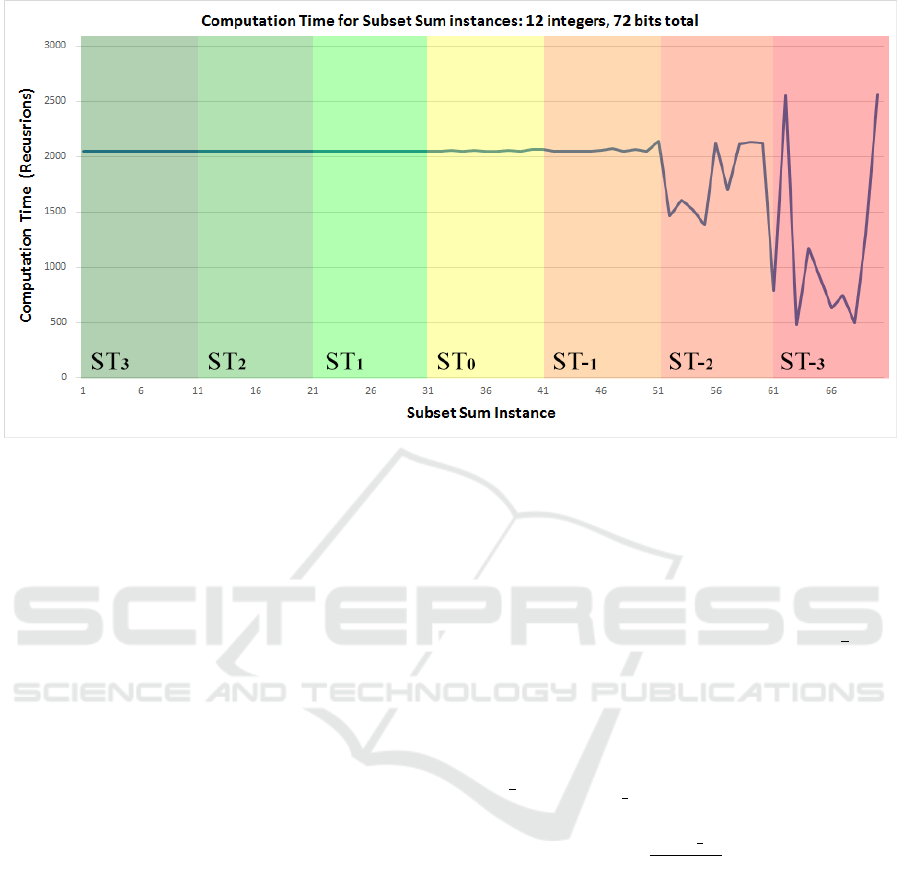
Figure 1: Strict templates of different eccentricity have different hardness patterns. Templates more eccentric than the linear
template ST
0
have no variation in computational hardness. Templates less eccentric than ST
0
have both harder and easier
instances.
4 INFORMATION THEORY
The template approach we are adopting in this pa-
per is motivated by an information theoretical analysis
of the subset sum problem and its instance hardness.
Earlier and related work can be found in (Adriaans
and Van Benthem, 2008; Adriaans, 2020b; Adriaans,
2020a).
Generally speaking, let S be a set of numbers
∈ N
+
, let target value t be a natural number, and let
the pair (S,t) be a corresponding instance of the sub-
set sum problem. Such an instance will, from an in-
formation theoretical perspective be hard if t contains
‘minimal’ information about the subsets of S. In other
words, suppose (S, t) is a yes-instance of subset sum
and (S,t
no
) is a no-instance, then it should be difficult
to distinguish these two: there should be no computa-
tional predicate (i.e. a computer program) that read-
ily identifies some structural difference between the
two. Using insights from information theory we can
argue that such instances exist, although we can never
construct them explicitly. The conditions we have to
create are prima facie simple:
1. The set S should have maximal entropy.
2. The numbers t and t
no
should have maximal en-
tropy given S.
In order to identify the numbers that satisfy the second
condition we can use the following lemma:
Lemma 4.1. Let S be a finite set of objects of cardi-
nality n. The maximal amount of conditional infor-
mation I(S
i
|S) in a subset S
i
⊂ S is n bits, for large
enough n, and it is reached when we select
1
2
n ele-
ments from S under uniform distribution.
Proof: When we select k objects from a set with cardi-
nality n, we need at most log
2
n
k
bits for an index of
this subset, since there are
n
k
of such subsets. New-
ton’s binomium is symmetrical and peaks at the value
k =
1
2
n with log
2
n
1
2
n
≈ n. Asymptotically we have:
lim
n→∞
log
2
n
1
2
n
n
= 1
If we use a Bernoulli process (i.e. coin flipping) to se-
lect the elements of S
i
we may, without loss of gener-
ality, assume that it has maximal conditional entropy.
In order to understand how Lemma 4.1 can be used to
identify hard cases of subset sum, we first turn our at-
tention to exemplars that have very low entropy: sets
that contain only powers of two. Equation 1 illustrates
the special nature of these sets:
Σ
n
i=0
2
i
= 2
n+1
− 1 (1)
Furthermore, it will prove useful to define the notion
of the scale of a number:
Definition 4.2. The scale of a number n ∈ N
+
is given
by sc(n) = dlog
2
(n)e.
Subset Sum and the Distribution of Information
137

The scale of a binary number is related to the number
of bits we need to encode it. We observe that, when
S consists only of powers of two, any corresponding
subset sum problem instance (S, t) is trivial and can
be solved in polynomial time. We can simply use
Equation 1 to estimate the scale of the target number t
and estimate its constituents. This procedure is analo-
gously effectuated by our branch and bound on strict
template ST
0
as found in Table 1. There is nothing ob-
scure about this: positional number systems are based
on the fact that any numbers can be easily rewritten as
the sum of the powers of the base (in this case 2). We
use this trivial concept every day from the moment we
learn elementary arithmetic (in this case base 10).
Next, we define the set of powers of two, ranging
from 2
0
to 2
n
as the scale-free reference set SF
n
:
Definition 4.3. The scale-free reference set SF
n
=
{2
i
|0 ≤ i ≤ n}.
Observe that we have Σ
x∈SF
n
x = 2
n+1
− 1. Note
that we can interpret the set SF
n
as a set of numbers
with typical scales and we can interpret Equation 1
as marking a scale transition: the scale of a number
n is associated with the largest set of powers of two
that sums up to a value smaller than n. Things get
interesting with the following theorem:
Theorem 4.4. The set of sums associated with subsets
of SF
n
with maximal entropy is scale-free.
Proof: Take set SF
n
, and apply lemma 4.1. A subset
SF
0
n
⊂ SF
n
with maximal entropy has ≈
1
2
n elements,
but there is no element of any scale from SF
n
that is
guaranteed to be in SF
0
n
. By equation 1, the scale of
Σ
x∈SF
0
n
x is not fixed over the set of subsets of SF
n
with
maximal conditional information.
The down-to-earth version of theorem 4.4 tells us
that when we use uniform distributions to select sub-
sets of SF
n
with maximal entropy, then the sums re-
sulting from these sets can have any value. To put
it even more simply: random numbers selected with
reference to a scale-free set can have any value, large
or small. The reverse of this result motivates the fol-
lowing observation:
Lemma 4.5. Let SF be a scale-free set, let t be a
target value and let (SF,t) be a corresponding sub-
set sum problem instance, then sc(t), the scale of t,
gives no indication about the conditional complexity
I(t|SF) of t.
Proof: Immediate consequence of lemma 4.4.
We can now use Lemma 4.5 to generate instances
of subset sum that, from an information theoretical
perspective, are hard. Instead of using the low com-
plexity set SF
n
= {2
i
|0 ≤ i ≤ n} we use a set with bit
templates of every scale:
Definition 4.6. A randomized linear scale free set
SF
r
n
of binary numbers of order n is a set of n ran-
dom binary numbers with for each i ∈ N ≤ n exactly
one number with a representation of i bits.
Such sets
• are still scale-free, so lemma 4.5 applies: let SF
r
n
be a randomized linear scale-free set and t a num-
ber in a reasonable range [0,
1
2
n(n + 1)] then the
size of t does not give any information about its
conditional complexity.
• have maximal entropy. We could use any random
string of length
1
2
n(n+1) bit to generate a set with
n elements by simply cutting the string in n seg-
ments of increasing length.
• when used as a template, produce subset sum
problem instances that are constraint-free. Every
random string of sufficient length defines an in-
stance of the problem class.
• have high average case complexity, by the same
reasoning.
• contain random numbers, and consequently are
always between 2
i
and 2
i+1
for some value of i.
Thereby, the conditions of equation 1 are not satis-
fied: the sums that can be constructed on the basis
of subsets of SF
r
n
will have holes and doubles on
any scale. Differently put: yes- and no-instances
for target values t will be mixed at every reason-
able scale.
With the definition of the concept of randomized lin-
ear scale free sets we have reached our goal of defin-
ing a class of subset sum problems that are hard from
an information theoretical point of view:
1. The sets SF
r
n
have maximal entropy.
2. There are yes-instances (SF
r
n
,t) and no-instances
(SF
r
n
,t
no
) for which the numbers t and t
no
have
maximal conditional entropy given SF
r
n
.
This result does not in itself prove that subset sum
problems based on scale-free templates are algorith-
mically hard, but it does explain the results of the
small experiment we report in this paper, and the piv-
otal role of the ST
0
set. We expect the phase transition
marked by scale-free sets to be more expressive when
larger examples are analyzed.
5 DISCUSSION
It seems that the distribution of informational bits
among the integers in a subset sum instance can play
a critical role in its experimental hardness. Each of
ECTA 2021 - 13th International Conference on Evolutionary Computation Theory and Applications
138

the 70 instances solved in this study, had n = 12 inte-
gers, and m = 78 input bits – no exceptions. But the
distribution of informational bits over the input ele-
ments was very different, and that seems to make a
huge difference.
Part of the hardness differentiation might be due
to the intrinsically binary nature of our branch and
bound algorithm, which decides on including or ex-
cluding a single element at the time. For very skewed
information distributions, as found in the random
instances generated by eccentric strict templates, it
thereby allows to discard half the search tree from the
root, effectively halving the runtime. There is even
a situation conceivable in which every non-discarded
subtree can also be split into directly discardable sub-
trees. For these numbers of bits and integers, it is the
set {1, 2, 4, 8...2048}, a special ‘maximal’ instance
from template ST
0
, which is likely the easiest ex-
istable instance in our experiment. From an infor-
mational theoretical perspective however, scale-free
non-strict templates can be used to generate hard sub-
set sum instances.
6 FUTURE WORK
There has been a lot of research on instance
hardness for various NP-complete problems, such
as SAT, K-colorability, VLSI routing and rect-
angle packing (Cheeseman et al., 1991)(Mitchell
et al., 1992)(Mu and Hoos, 2015)(Kirkpatrick and
Selman, 1994)(Turner, 1988)(Hogg and Williams,
1994)(Venkatesan and Levin, 1988)(Jansen et al.,
2020)(van den Berg et al., 2016)(Pejic and van den
Berg, 2020).
For the Hamiltonian cycle problem, also NP-
complete, there seems to be an interesting similar-
ity with this study. Although in completely random
ensembles, the hardest instances are located in an
area around the Koml
´
os-Szemer
´
edi bound (Cheese-
man et al., 1991)(van Horn et al., 2018)(Koml
´
os and
Szemer
´
edi, 1983)(Sleegers and Berg, 2021), an un-
informed heuristical search found the hardest prob-
lem instances in a very edge-dense region (Sleegers
and van den Berg, 2020b)(Sleegers and van den Berg,
2020a). The most interesting similarity in results
however, is that in this edge-dense region, the hard-
est and easiest Hamiltonian cycle problem instances
were very close together, separated by just one bit
of information. Could it be that the Hamiltonian cy-
cle instances in the edge-dense region have some-
thing in common with NP-complete subset sum in-
stances generated through flat templates? With some
imagination, both areas could be seen as ‘low entropy
plains’, dense in solutions, but punctured with numer-
ous very small very deep holes in which very hard
instances live – instances that have no solutions, and
voraciously devour algorithmic recursions while try-
ing to find one.
There is also some relevant work on instance hard-
ness for NP-hard optimization problems. Most rel-
evant might be studies on the asymmetric traveling
salesman problem. The standard deviation in the dis-
tance matrix generation procedure turned out to be
an unreliable predictor of instance hardness (Cheese-
man et al., 1991)(Sleegers et al., 2020), but a later
study by WeiXiong Zhang and Richard Korf, solved
their ATSP instances with a branch and bound algo-
rithm similar, but not identical, to ours (Zhang and
Korf, 1996). They didn’t use (strict) templates, but
did something very similar, drawing their matrix en-
tries from {0, 1, 2...r}. Their finding, and this is really
interesting, is a ‘complexity transition’ similar but not
identical to ours, and their explanation of the control-
ling factor: the number of distinct entries in the ma-
trix. Are we again looking at instance entropy as a
predictive data analytic for instance hardness? Less
diverse entries in a subset sum instance means fewer
different outcomes too, but the difference between
‘less’ and ‘fewer’ is so mysterious in this context that
we dare not speculate any further. We need more evi-
dence, so as for the future, it looks like we’ve got our
work cut out for us.
ACKNOWLEDGEMENTS
We would like to thank the IvI Complex Cyber Infras-
tructure (CCI) group and its director Cees de Laat for
their support.
REFERENCES
Adriaans, P. (2020a). A computational theory of meaning.
Advances in Info-Metrics: Information and Informa-
tion Processing across Disciplines, page 32.
Adriaans, P. (2020b). Information. In Zalta, E., edi-
tor, The Stanford Encyclopedia of Philosophy. Meta-
physics Research Lab, Stanford University, fall 2020
edition.
Adriaans, P. and Van Benthem, J. (2008). Philosophy of
information. Handbook of the Philosophy of Science,
(8).
Brickell, E. F. (1984). Solving low density knapsacks. In
Advances in cryptology, pages 25–37. Springer.
Cheeseman, P., Kanefsky, B., and Taylor, W. M. (1991).
Where the Really hard problems are. In IJCAI, vol-
ume 91, pages 331–340.
Subset Sum and the Distribution of Information
139

Daan van den Berg (2019). Refurbished version of Lital’s
paper. http://www.heuristieken.nl/resources/(1963)
Littleetal- refurbished AlgorithmforTSP.pdf. Last ac-
cessed june 18
th
, 2021.
Eastman, W. L. (1958). Linear programming with pattern
constraints: a thesis. PhD thesis, Harvard University.
Garey, M. R. and Johnson, D. S. (1979). Computers and
intractability, volume 174. freeman San Francisco.
Hogg, T. and Williams, C. P. (1994). The hardest constraint
problems: A double phase transition. Artificial Intel-
ligence, 69(1-2):359–377.
Jansen, R., Vinkesteijn, Y., and van den Berg, D. (2020).
On the solvability of routing multiple point-to-point
paths in manhattan meshes. In Proceedings of the
2020 Genetic and Evolutionary Computation Confer-
ence Companion, pages 1685–1689.
Kemal Tural, M. (2020). On the hardness of almost all
subset sum problems by ordinary branch-and-bound.
arXiv, pages arXiv–2001.
Kirkpatrick, S. and Selman, B. (1994). Critical behavior in
the satisfiability of random boolean expressions. Sci-
ence, 264(5163):1297–1301.
Koml
´
os, J. and Szemer
´
edi, E. (1983). Limit distribution for
the existence of hamiltonian cycles in a random graph.
Discrete Mathematics, 43(1):55–63.
Lagarias, J. C. and Odlyzko, A. M. (1985). Solving low-
density subset sum problems. Journal of the ACM
(JACM), 32(1):229–246.
Land, A. and Doig, A. (1960). An automatic method of
solving discrete programming problems. Economet-
rica, 28(3):497–520.
Land, A. H. and Doig, A. G. (2010). An automatic method
for solving discrete programming problems. In 50
Years of Integer Programming 1958-2008, pages 105–
132. Springer.
Little, J. D., Murty, K. G., Sweeney, D. W., and Karel, C.
(1963). An algorithm for the traveling salesman prob-
lem. Operations Research, 11(6):972–989.
Mitchell, D., Selman, B., and Levesque, H. (1992). Hard
and easy distributions of SAT problems. In AAAI, vol-
ume 92, pages 459–465.
Mu, Z. and Hoos, H. H. (2015). On the empirical time
complexity of random 3-sat at the phase transition. In
Twenty-Fourth International Joint Conference on Ar-
tificial Intelligence.
Pejic, I. and van den Berg, D. (2020). Monte carlo
tree search on perfect rectangle packing problem in-
stances. In Proceedings of the 2020 Genetic and Evo-
lutionary Computation Conference Companion, pages
1697–1703.
Rossman, M. and Twery, R. (1958a). Combinatorial-
programming. In OPERATIONS RESEARCH,
volume 6, pages 634–634. INST OPERATIONS
RESEARCH MANAGEMENT SCIENCES 901
ELKRIDGE LANDING RD, STE . . . .
Rossman, M. and Twery, R. (1958b). A solution to
the traveling salesman problem by combinatorial-
programming. In Operations Research, volume 6,
pages 897–897. INST OPERATIONS RESEARCH
MANAGEMENT SCIENCES 901 ELKRIDGE
LANDING RD, STE . . . .
Skiena, S. S. (1998). The algorithm design manual. page
247.
Sleegers, J. and Berg, D. v. d. (2021). Backtracking (the)
algorithms on the hamiltonian cycle problem. arXiv
preprint arXiv:2107.00314.
Sleegers, J., Olij, R., van Horn, G., and van den Berg, D.
(2020). Where the really hard problems aren’t. Oper-
ations Research Perspectives, 7:100160.
Sleegers, J. and van den Berg, D. (2020a). Looking for
the hardest hamiltonian cycle problem instances. In
IJCCI, page 40–48.
Sleegers, J. and van den Berg, D. (2020b). Plant propa-
gation & hard hamiltonian graphs. In Evostar 2020
“The Leading European Event on Bio-Inspired Com-
putation”.
Turner, J. S. (1988). Almost all k-colorable graphs are easy
to color. Journal of algorithms, 9(1):63–82.
van den Berg, D., Braam, F., Moes, M., Suilen, E., and Bhu-
lai, S. (2016). Almost squares in almost squares: Solv-
ing the final instance. Data Analytics 2016, page 81.
van Horn, G., Olij, R., Sleegers, J., and van den Berg, D.
(2018). A predictive data analytic for the hardness of
hamiltonian cycle problem instances. Data Analytics
2018, page 101.
Venkatesan, R. and Levin, L. (1988). Random instances of
a graph coloring problem are hard. In Proceedings
of the twentieth annual ACM symposium on Theory of
computing, pages 217–222.
Zhang, W. and Korf, R. E. (1996). A study of complex-
ity transitions on the asymmetric traveling salesman
problem. Artificial Intelligence, 81(1-2):223–239.
ECTA 2021 - 13th International Conference on Evolutionary Computation Theory and Applications
140
