Formulation of Multifactorial Regression Model of Life Expectancy

based on Correlation and Regression Analysis

Kristina Salnikova

and Rinat Faizullin

Institute of Digital Economy, Kalashnikov ISTU, Izhevsk, Russia

Management Technologies, MIREA — Russian Technological University, Moscow, Russia

Keywords: Correlation Analysis, Correlation Coefficient, Matrix of Correlation Interfactor Coefficients, Life

Expectancy, Multicollinearity, Heteroscedasticity, Econometric Model.

Abstract: The paper considers the formulation of a multifactorial regression model to study life expectancy dependence

on 11 factors (GDP per capita according to purchasing power parity (PPP) in US dollars; prevalence of any

type of tobacco use among women over 15 (cigarettes, pipes, hookah, etc.) as percentage of the total female

population over 15 years of age; prevalence of any type of tobacco use among men over 15 as percentage of

the total male population over 15 years of age; diabetes risk as percentage for the population from 20 to 79

years old; Gini index; number of children who died under 1 year of age; air pollution with PM2.5 particles (in

micrograms per cubic meter) per capita; health expenditure as percentage of GDP; health expenditure per

capita; annual consumption of pure alcohol per capita for the population over 15 years of age; amount of

population over 65 years of age; household consumption in US dollars for further modeling and forecasting

in decision-making. The aim presented in the paper consists in obtaining information about the type and extent

of relationship between life expectancy and factors, exclusion of insignificant factors and formulation of the

econometric model. The authors used R-Studio language to achieve this goal.

1 INTRODUCTION

Econometric models reflect statistic patterns, the

purpose of which is to use quantitative analysis and

forecast of the relationships of indicators describing

an economic object to prepare and make informed

economic decisions. There are software products that

can potentially be used to formulate a multifactorial

regression model and not only, such as MS Excel,

Gretl, SPSS, STATA, Eviews, R.

In recent years, many works on this topic have

been published by authors from Russia, both on the

assessment of the influence of many factors on life

expectancy (Zvezdina and Ivanova, 2015;

Merkushova, 2015; Mironova, 2020, Shibalkov and

Nedospasova, 2020), and on the influence of

individual factors, e.g., the impact of alcohol

consumption on life expectancy in Russia (Kossova

et al., 2017), on gender and regional differences in life

expectancy in Russia (Rodionova and Kopnova,

2020).

https://orcid.org/0000-0002-2780-8857

https://orcid.org/0000-0002-1179-3910

There are also works that study life expectancy in

different countries (Kontis V. et al., 2017), influence

of factors on early mortality (Platt O. S. et al., 1994).

The influence of a single factor on life expectancy in

a particular country during a certain period is often

investigated. For instance, P. T. Katzmarzyk & I. M.

Lee (Katzmarzyk and Lee, 2012) describe the impact

of sedentary lifestyle on life expectancy in the United

States, and J. E. Bennett (Bennett J. E. et al., 2019)

estimates the impact of air pollution with solid

particles on life expectancy in the United States.

In this paper, it is proposed to illustrate the

formulation of a multifactorial regression model of

life expectancy dependence based on the use of

correlation and regression analysis apparatus,

applying a correlation matrix based on the correlation

coefficients between all available factors and

exclusion of variables that are not significant for the

model.

306

Salnikova, K. and Faizullin, R.

Formulation of Multifactorial Regression Model of Life Expectancy based on Correlation and Regression Analysis.

DOI: 10.5220/0010667700003223

In Proceedings of the 1st International Scientiﬁc Forum on Sustainable Development of Socio-economic Systems (WFSDS 2021), pages 306-312

ISBN: 978-989-758-597-5

2 METHODOLOGY

Correlation analysis is a method of mathematical

statistics used to study and investigate the relationship

between (general) economic indicators based on their

observed statistic (sample) analogs.

Paired correlation analysis is the study of the

relationship between two economic indicators that

describe the properties of the same type of objects

from a certain population. Consequently, the paired

correlation analysis is one of the tools for selecting

factors for the regression model and selecting the

form of relationship between the dependent variable

and determining factors. Using this method, you can

check the relevance of some selected factors for this

model. In order to draw conclusions about the mutual

dependence of the selected indicators, it is necessary

to build correlation fields and analyze the locations of

points on them. If the points are located

approximately on the same straight line and have

slight deviations in both directions from it, then we

can talk about the presence of linear relationship. The

type of relationship can be determined by the straight

line slope. It can be direct or reverse. If it is possible

to trace a certain curvature of the band of points on

the graph, then we can talk about the presence of

nonlinear dependence between the indicators. And

when the points are scattered over a certain area, it

can be stated that there is no correlation. Based on the

graphical analysis, it is necessary to make a visual

assessment and present the data in the form of the

correlation field.

The relationship graphical description consists in

constructing an empirical regression line that

connects the points on the correlation field, the

abscissae of which are the values of the attribute-

factor (individual or group), and the ordinates are the

average values of the resulting attribute.

As researches demonstrate (Salnikova, 2020), the

relationship strength is assessed using the correlation

indicators:

1. K. Pearson linear coefficient of paired

correlation (r



 evaluates the strength and direction

of only linear relationship between two attributes

calculated by formulas (1), (2) and (3):

𝑟





∑













∙















(1)

𝑟











∙







∙



(2)

𝑟







∑



∑



∑







∑







∑





∙

∑







∑







(3)

where 𝜎



and 𝜎



- standard deviations of factorial

and resultant attributes;

x and y - values of the attributes.

The value of the linear correlation coefficient is

within (formula (4):

1  r



 1 (4)

1) if 𝑟



1, the relationship is functional, i.e.

ratio y=a+bx is fulfilled for all observations:

- if 𝑟



1, the relationship is direct (𝑏

0, which means functional relationship between 𝑥

and 𝑦;

- if 𝑟



1, the relationship is reverse

(𝑏0;

2) if r = 0, there is no linear relationship, but there

may be a nonlinear one;

3) if 0𝑟1, the relationship is direct (y

increases with x increase);

4) if 1  𝑟  0, the relationship is reverse (y

decreases with x increase).

The closer the absolute value of 𝑟



 is to 1, the

stronger the linear relationship is and the better the

linear relationship agrees with the observation data.

Any intermediate value of 𝑟 from 0 to 1 characterizes

the degree of approximation of the correlation

relationship between 𝑥 and 𝑦 to the functional one.

To determine the relationship strength between

the indicators, it is necessary to build a matrix of

interfactor correlation coefficients.

The aim of the work is to study the dependence of

life expectancy based on the use of the apparatus of

correlation-regression analysis. Next, we will build a

regression model of the dependence of life

expectancy in all countries of the world on the value

of the value of various factors in 2015. and see how

much it has changed in 2020. Since life expectancy

depends on various factors: income level, lifestyle,

education, heredity, ecology, nutritional quality,

development of the health care system and others.

Then, to build a predictive econometric model, we

take 11 factors (World Health Organization):

 gdppc - GDP per capita according to PPP in US

dollars;

 smokingfemale - prevalence of any type of

tobacco use among women over 15 (cigarettes,

pipes, hookah, snus, etc.) as percentage of the

total female population over 15 years of age;

 smokingmale - prevalence of any type of tobacco

use among men over 15 as percentage of the total

male population over 15 years of age;

 diabetes - diabetes risk as percentage for the

population from 20 to 79 years old;

 gini - Gini index;

 childdeath - number of children who died under

1 year of age;

Formulation of Multifactorial Regression Model of Life Expectancy based on Correlation and Regression Analysis

307

 airpollution - air pollution with PM2.5 particles

(in micrograms per cubic meter) per capita;

 healthexpenditure - health expenditure as

percentage of GDP;

 healthexpenditure1 - health expenditure per

capita;

 alcohol - annual consumption of pure alcohol per

capita for the population over 15 years of age;

 undersixtyfive - amount of population over 65

years of age;

 hconsump - household consumption in US

dollars.

Let us find a set of factors that should be included

in the regression model, and also identify those that

are insignificant (do not affect the dependent variable

value). We also find the type of dependence between

the dependent variable and predictors.

The purpose of correlation analysis is to obtain

information about the type and extent of relationship

between life expectancy and factors.

Determination of the type and extent of

correlation relationship between life expectancy

and factors.

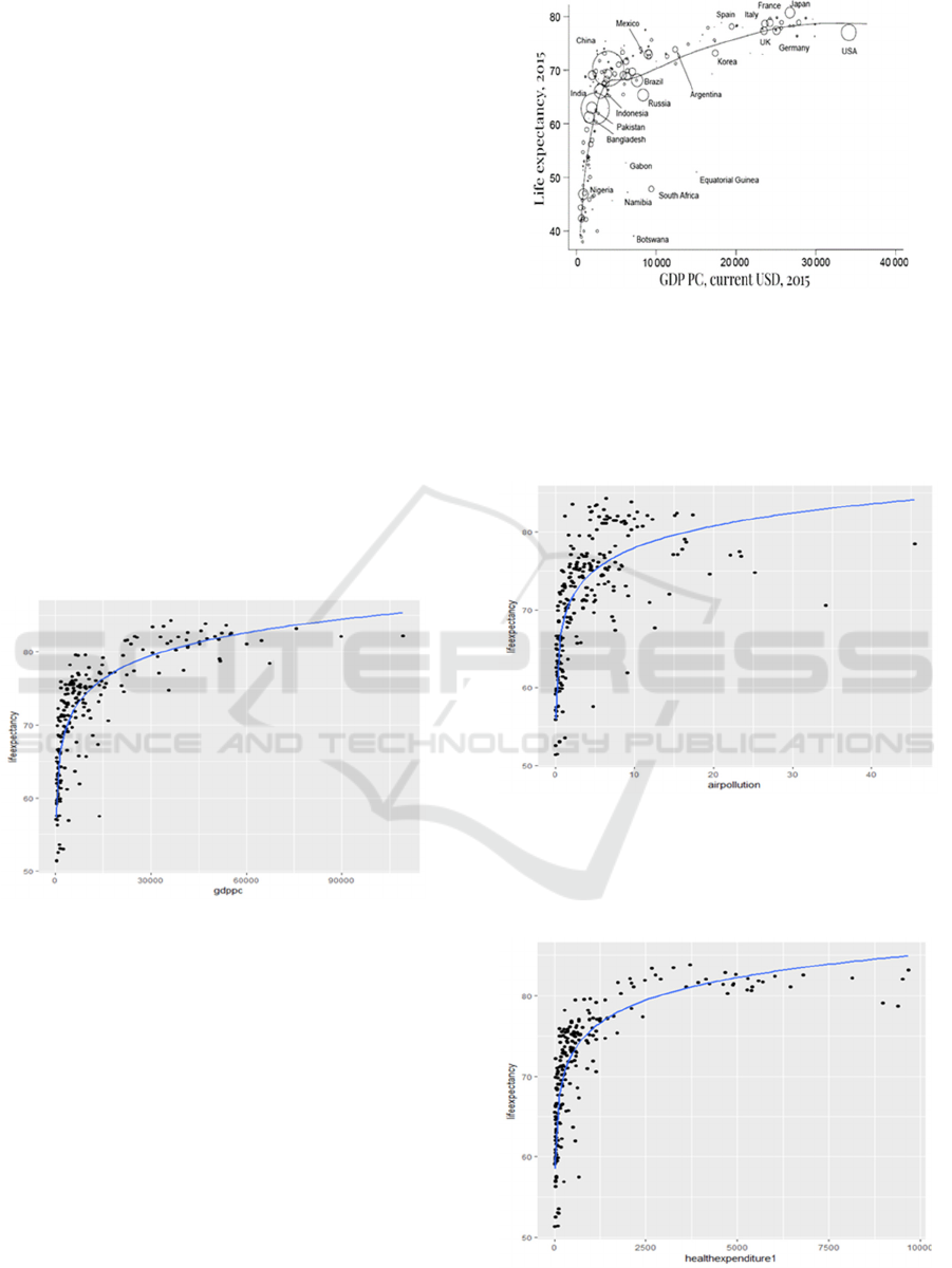
Figure 1: Correlation field of lifeexpectancy & gdppc.

Below are the graphs of the correlation field for

all factors.

In Figure 1, the graph demonstrates direct linear

correlation dependence between GDP level per capita

in prices of 2015. This dependence is also called

Preston Curve and has been around for about 100

years, so it is often mentioned in medical researches.

The dependence shows that a person born in a rich

country can, on average, according to forecasts live

longer than a person born in a poor country. As

income increases, life expectancy goes up, but after

60,000 US dollars per person life expectancy growth

slows down.

Countries can be located above or below Preston

Curve. For instance, SAR is far below the curve,

Figure 2: Correlation field of life expectancy & GDP PC/2.

meaning that life expectancy is much lower than the

potential one at the current income level. At the same

time, Mexico is above the curve, which means that

life expectancy is higher than the average for the

given income level (Figure 2).

Figure 3: Correlation field of lifeexpectancy & airpollution.

The third graph in Figure 3 demonstrates

contradictory results, so we will later eliminate the air

pollution factor.

Figure 4: Correlation field of lifeexpectancy &

smokingfemale.

WFSDS 2021 - INTERNATIONAL SCIENTIFIC FORUM ON SUSTAINABLE DEVELOPMENT OF SOCIO-ECONOMIC SYSTEMS

308

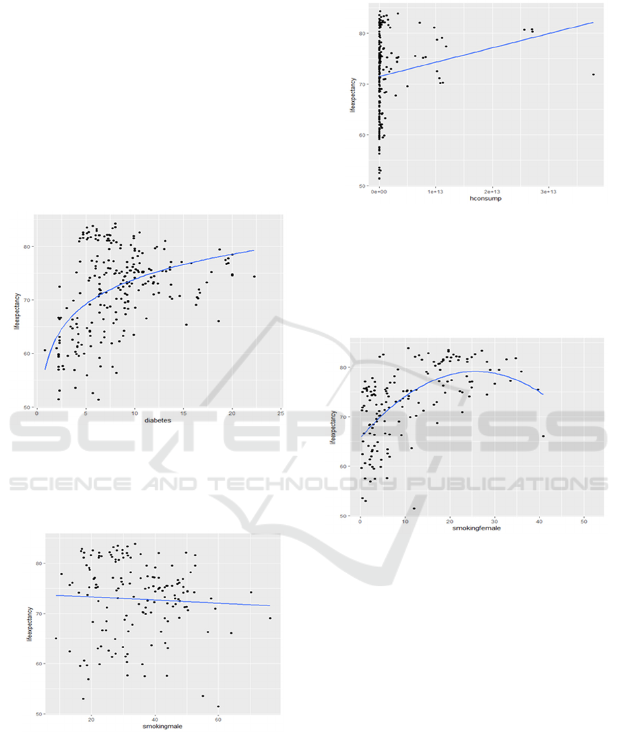
Mathematically, this graph in Figure 4 means that

the first derivative of the life expectancy function is

positive depending on the proportion of smoking

women, but it decreases, and the second one is

negative. In other words, the function increases and is

convex upwards.

The derivative of the life expectancy function

dependence on the proportion of smoking women

(derivative) decreases with an increase in the

proportion of smoking women, and turns to zero at

the maximum life expectancy and then becomes

negative, and life expectancy, having reached the

maximum value, begins to decrease.

Figure 5: Correlation field of lifeexpectancy &

smokingmale.

According to the graph in Figure 5, there is

negative dependence between the life expectancy and

number of smoking men, but the dependence is weak.

Figure 6: Correlation field of lifeexpectancy & diabetes.

The dependence turns out to be contradictory, and

it is impossible to give full interpretation (Figure 6).

A possible explanation can be found in the fact that in

countries where food is better, the diabetes rate is

higher. However, the life expectancy is higher in the

same countries.

Figure 7: Correlation field of lifeexpectancy &

healthexpenditure1.

According to the World Health Organization,

there is direct dependence between total health

expenditure (per capita) and life expectancy.

From the graph in Figure 7 we can conclude that

this statement is correct.

Figure 8: Correlation field of lifeexpectancy & hconsump.

Thus, it can be seen that there is no dependence

between life expectancy and household consumption

(Figure 8).

Let us prepare a correlation matrix based on the

correlation coefficients between all available

variables (Figure 9):

Formulation of Multifactorial Regression Model of Life Expectancy based on Correlation and Regression Analysis

309

Figure 9: Correlation matrix based on the correlation

coefficients between all available variables for 2015.

From the data in Figure 9 it can be seen that the

correlation dependence between life expectancy and

factorial variables does not exist everywhere. This

table confirms the assumptions expressed on the

graphical analysis basis.

Determination of the extent of mutual

influence on life expectancy of all factors

𝑅



 0.6235

We can conclude that the change in life

expectancy by 62.35% is due to the change in the

factors included into the model.

Let us check the combined influence of the factors

on life expectancy, calculated by formula (5):

𝐹

























(5)

where

𝑅



– determination coefficient (square of multiple

correlation coefficient), 𝑅





Multiple R  Squared





0.6235

𝑛 – sample size, 𝑛  264  108  156 , 108

observations deleted due to missingness,

𝑘 – number of predictors, 𝑘5

𝐹





0.6235 ∙



156  5 1





1  0.6235



∙5

 49.681

𝐹





5;150;0,05



 4.3650

Since 𝐹



𝐹



, consequently, with 95%

probability, together the factors significantly affect the life

expectancy.

In comparison with the data for 2020, the

correlation dependence between the life expectancy

and factorial variables does not exist everywhere, as

well as in the correlation matrix based on the

correlation coefficients for 2015.

Therefore, it is proposed to exclude variables that

are not significant for the model based on the data

array used. After identifying significant factors using

t-statistics, there were suspicions about the existence

of multicollinearity between the two factors: gdppc

and healthexpenditure1, as the graphical analysis

contradicted the results of the t-statistics check. VIF

test is used to check the factors for multicollinearity.

Results of the test conducted in R-Studio (Table

1):

Table 1: VIF test.

Gdppc 16.384332

Healthexpenditure1 18.906159

Smokingmale 1.709373

smokingfemale 1.702277

diabetes 1.212224

gini 1.909564

hconsump 2.075939

alcohol 1.722765

childdeath 1.353089

As you can see, there is high multicollinearity

between gdppc and healthexpenditure1, that is,

pairwise correlation dependence between the factors.

This means that one of these factors should be

eliminated.

Variable elimination method - used to eliminate

multicollinearity. It consists in removing highly

correlated explanatory variables from the regression

and reevaluating it.

The selection procedure for the main factors

includes the following steps:

1. The analysis of the values of the coefficients of

pair correlation 𝑟









between the factors 𝑥



and 𝑥



carried out.

2. The identified pairwise-dependent factors are

analyzed according to the closeness of the

relationship between the explanatory factors and the

effective variable.

If we exclude healthexpenditure1 from the model,

then 𝑅





Adjusted



 0.6254. If we exclude gdppc

from the model, then 𝑅





Adjusted



 0.6121. So, it

makes more sense to exclude healthexpenditure1

from the model.

Now, after conducting VIF test, we can exclude

the remaining insignificant factors from the model,

such as: alcohol, hconsump. At the same time,

𝑅





Adjusted



will increase up to 0.649.

WFSDS 2021 - INTERNATIONAL SCIENTIFIC FORUM ON SUSTAINABLE DEVELOPMENT OF SOCIO-ECONOMIC SYSTEMS

310

3 RESULTS

After passing all the analysis stages, our econometric

model takes the following form:

lifeexpectancy  3.43 ∙ loggdppc  2.94

∙ logdiabetes  0.09719 ∗ gini

The factors such as the percentage of smoking

women (smokingfemale), child mortality

(childdeath) were excluded from the model after

checking the significance of regression coefficients

based on t-statistics.

According to VIF test, the model is not

multicollinear (Table 2).

Table 2: VIF-test.

log(gdppc) log(diabetes) gini

1.232833 1.035453 1.211515

Heteroscedasticity was revealed in the model.

After adjusting for heteroscedasticity, the gini factor

was insignificant. However, if we exclude it from the

model, R





adj



will decrease from 0.8 to 0.71, which

significantly affects the model quality.

Moreover, the heteroscedasticity in our model is

very weakly expressed, this is evidenced by a rather

high 𝑝 𝑣𝑎𝑙𝑢𝑒0.01104. So, it was decided to

leave the gini factor in the model.

With 95% probability, the factors that are

included into the model collectively have a

statistically significant effect on the change in

lifeexpectancy (the regression is generally

significant).

4 DISSCUSSION OF RESULTS

Most of the phenomena and processes in the economy

are closely related. Its identification and analysis is a

primary task at the initial stage of developing a

forecasting model. This allows us to discard

insignificant factors, to understand the process of

cause-and-effect relationships between factors. It is

very convenient to investigate dependencies using

correlation-regression analysis.

In light of the impact of COVID-19 on life of

people, the current topic of research is the forecast of

life expectancy, taking into account significant

factors and possibility of further development of the

necessary measures. The econometric model obtained

in the course of research shows that life expectancy

in a country depends on such factors as the gross

domestic product per capita, prevalence of diabetes

among the population, and Gini index.

5 CONCLUSION

So, the following stages of data analysis were

implemented:

 based on open statistic data, the set of 11 factors

that affect life expectancy was formed;

 insignificant factors were excluded from the

model: healthexpenditure1. Using the software

product, VIF test was performed in R-Studio to

check the factors for multicollinearity. The

insignificant factors were excluded from the

model, such as: alcohol, hconsump;

 econometric model was obtained and tested for

heteroscedasticity.

The resulting methodology can be applied in life

expectancy analysis, and can also be used by

specialists in the process of forecasting various

decisions in the adoption of regional policy.

REFERENCES

Bennett, J. E. (2019). Particulate matter air pollution and

national and county life expectancy loss in the USA: A

spatiotemporal analysis, PLoS medicine, 16: e1002856.

Katzmarzyk, P. T., Lee I. M. (2012). Sedentary behaviour

and life expectancy in the USA: a cause-deleted life

table analysis, BMJ open., 2(4).

Kontis, V. (2017). Future life expectancy in 35

industrialized countries: projections with a Bayesian

model ensemble, The Lancet, 389(10076): 1323-1335.

Kossova, T. V., Kossova, E. V., Sheluntsova, М. А. (2017).

Influence of alcohol consumption on mortality and life

expectancy in regions of Russia, Economic policy,

12(1).

Merkushova, N. I. (2015). Statistic analysis of population

life expectancy, Bulletin of Samara State Economic

University, 4: 102-109.

Mironova, А. А. (2020). Methodology for assessing the

load of mortality for different reasons onto life

expectancy, Human ecology, 5.

Platt, O. S. (1994). Mortality in sickle cell disease--life

expectancy and risk factors for early death., New

England Journal of Medicine, 330(23): 1639-1644.

Rodionova, L. A., Kopnova, E. D. (2020). Gender and

regional differences in life expectancy in Russia, Issues

of statistics, 27(1): 106-120.

Salnikova, K. V. (2020). Practical basics of statistics and

econometric modeling: study guide,

http://www.iprbookshop.ru/91121.html

Shibalkov, I. P., Nedospasova, O. P. (2020). Complex

assessment of the influence of social and economic

Formulation of Multifactorial Regression Model of Life Expectancy based on Correlation and Regression Analysis

311

factors on life expectancy of population in regions of

Russia, STT Publishing.

World Health Organization, Global Health Observatory

Data Repository, http://apps.who.int/ghodata/

Word Bank, World Development Indicators,

http://databank.worldbank.org/data/reports.aspx?sourc

e=2&series=AG.LND.AGRI.ZS&country=

Zvezdina, N. V., Ivanova, L. V. (2015). Life expectancy in

Russia and factors influencing it, Issues of statistics, 7:

10-20.

WFSDS 2021 - INTERNATIONAL SCIENTIFIC FORUM ON SUSTAINABLE DEVELOPMENT OF SOCIO-ECONOMIC SYSTEMS

312