Benzene Prediction: A Comparative Study of ANFIS, LSTM and
MLR
Andreas Humpe
1a
, Holger Günzel
2b
and Lars Brehm
2c
1
University of Applied Sciences Munich, Schachenmeierstrasse 35, 80636 Munich, Germany
2
University of Applied Sciences Munich, Am Stadtpark 20, 81243 Munich, Germany
Keywords: Prediction Model, Air Pollution, Benzene, Adaptive Neuro-Fuzzy Inference System, Long-Short-Term
Memory, Multiple Linear Regression.
Abstract: It is generally recognized that road traffic emissions are a major health risk and responsible for a substantial
share of death and disease in Europe. Although artificial intelligence methods have been used extensively for
air pollution forecasting, there is little research on benzene prediction and the use of long short-term memory
networks. Benzene is considered one of the pollutants of greatest concern in urban areas and has been linked
to leukemia. This paper investigates the predictive power of adaptive neuro-fuzzy inference systems, long
short-term memory networks and multiple linear regression models for one hour ahead benzene prediction in
the city of Augsburg, Germany. The results of the analysis indicate that adaptive neuro-fuzzy inference
systems have the best in sample performance for benzene prediction, whereas long short-term memory
networks and multiple linear regressions show similar predictive power. However, long short-term memory
models have the best out of sample performance for one hour ahead benzene prediction. This supports the use
of long short-term memory networks for benzene prediction in real emission forecasting applications.
1 INTRODUCTION
Recently, the European Environment Agency (EEA,
2020) announced that the single largest environmental
health risk and a major cause of premature death and
disease in Europe is air pollution. In urban areas, road
transport is the main contributor to emissions of
nitrogen dioxide (NO
2
) and benzene (C
6
H
6
) (for a
discussion see Krzyzanowski et al., 2005). Other
traffic related air pollutants include e.g. carbon
monoxide (CO), nitrogen monoxide (NO), ozone (O
3
)
and particu-late matter (PM10, PM2.5). Thus, traffic
induced air pollution is still a serious issue in many
large cities.
Heart disease, stroke, lung diseases and lung
cancer are the most common reasons for premature
death attributable to air pollution (European
Environment Agency, 2020). According to Künzli et
al. (2000) air pollution is responsible for more than 5%
of deaths in Europe and half of this can be attributed
to motor vehicles. Overall, European air quality has
improved in recent years, but is still too high (The
a
https://orcid.org/0000-0001-8663-3201
b
https://orcid.org/0000-0003-3410-1443
c
https://orcid.org/0000-0003-0810-3752
Lancet Commission, 2017). Consequently, there is a
need for air quality management and for tools to
quantify the effects of proposed and implemented
measures (European Environment Agency, 2019).
Benzene is considered one of the pollutants of
most concern in urban areas that is associated with
various diseases (De Donno et al., 2018 and Smith,
2010). Benzene is included in the gasoline for motor
vehicles. For instance, when a car is refuelled,
benzene evaporates from the tank of the car and an
aromatic odour can be perceived. However, the escape
of benzene during refuelling has been solved in recent
years by "gas displacement". Nevertheless, the main
part of the pollution is due to road traffic. Benzene is
a component of the escaping exhaust gases from the
tailpipe (German Federal Environment Agency,
2021).
In June 2021 the Court of Justice of the European
Union ruled that Germany has breached EU laws by
failing to limit poor air quality. The European
Commission accused German authorities of not taking
enough action to comply with EU air pollution limits
318
Humpe, A., Günzel, H. and Brehm, L.
Benzene Prediction: A Comparative Study of ANFIS, LSTM and MLR.
DOI: 10.5220/0010660900003063
In Proceedings of the 13th International Joint Conference on Computational Intelligence (IJCCI 2021), pages 318-325
ISBN: 978-989-758-534-0; ISSN: 2184-3236
Copyright © 2023 by SCITEPRESS – Science and Technology Publications, Lda. Under CC license (CC BY-NC-ND 4.0)

and the Court of Justice of the European Union now
confirmed this appraisal (Court of Justice of the
European Union, 2021). In order to limit traffic
induced air pollution, it is necessary to implement
good forecasting tools. With the ability to predict air
pollution in advance, traffic management systems can
limit exhausts by limiting access of motor vehicles to
city centres. For this reason, the present research work
investigates which machine learning algorithms are
particularly well suited for the prediction of benzene,
as one of the most toxic exhaust gases in road traffic.
The results here should be of interest to academic and
traffic management authority alike who are concerned
with reducing air pollution by traffic control based on
accurate forecasting.
Artificial intelligence (AI) has been one of the
advanced tools for modelling and forecasting air
quality. For instance, Kaur et al. (2020) applied four
different artificial neural networks (ANN) to predict
PM2.5 concentration at hotspots in the city of Delhi.
The authors conclude that ANNs are well suited for
PM2.5 prediction and that the non-linear
autoregressive network with exogenous input
(NARX) outperforms other ANNs in step ahead
prediction. Similarly, Sayeed et al. (2020) makes use
of a deep convolutional neural network (CNN) to
predict ozone concentration. The model predicts
ozone concentration 24 hours in advance with great
accuracy and according to the authors, might be used
as an early warning system for individuals susceptible
to ozone. Further examples of successful ANNs
applications for air quality forecasting include
Molina-Cabello (2019) and Pawlak (2019).
In contrast, Ly et al. (2019) apply an adaptive
neuro-fuzzy inference system to predict NO
2
and CO
from multisensor and weather data in an unnamed
Italian city. They show that combining multioutput
sensor data with ANFIS techniques offers a powerful
way to model nonlinear processes such as air quality.
Others that have concluded that ANFIS models are
well suited for air pollution prediction include Ausati
et al. (2016), Mihalache et al. (2016), Oprea et al.
(2017) and Humpe et al. (2021).
Furthermore, decision tree methods have been
used to forecast air pollution by inter alias Loya et al.
(2012) or Lee et al. (2019). Overall, it has been
concluded that decision trees are quite helpful to
illustrate dependencies, but not particularly accurate
in forecasting compared to other methods.
More recently, long short-term memory networks
(LSTM) have been applied to pollution forecasting.
For instance, Bai et al. (2019) has used LSTM for
hourly PM2.5 concentration forecasting. Similarly,
Chang et al. (2020) apply LSTM models for
forecasting various air pollutants. Generally, the
literature on the use of LSTM models for forecasting
road traffic emissions is rather limited. In contrast to
standard recurrent neural networks (RNN) the long
short-term memory network (LSTM) considers both,
the short-term as well as long-term dependency of a
time series. Thus it has the advantage that it exhibits
temporal dynamic behaviour for a time sequences
(Greff et al., 2016). As emissions are characterised by
dynamic behaviour, LSTM networks might be
particularly useful in emission forecasting.
Furthermore, benzene forecasting research is also
underrepresented although benzene is considered one
of the pollutants of most concern in urban areas and
can be associated with acute myeloid leukemia,
myelodysplastic syndromes and lymphoma and
childhood leukemia (De Donno et al., 2018 and Smith,
2010). An exception to this is Karakitsios et al. (2006)
who predicted benzene concentration in a street
canyon using artificial neural networks. This paper
adds to the literature by analysing benzene concentra-
tion in the German city Augsburg and applying LSTM
networks. The results are expected to contribute to a
better understanding of benzene air pollution in the
future. This in turn might be used in traffic regulation
to improve air quality in cities and towns.
In a related article, Humpe et al. (2021) investigate
air pollution in Munich with a similar data set and
methodology. However, benzene as one of the most
worrisome pollutants is not measured and recorded for
the city of Munich. This article therefore extends the
study by analysing another hazardous traffic pollutant
that has been recorded for the city of Augsburg.
Furthermore, in comparison to the earlier study this
article includes LSTM networks that might be
particularly suited to forecast out of sample benzene
concentration due to their ability to forget part of its
previously stored memory and at the same time also
add a part of new information.
2 MATERIAL
This research used hourly data of benzene, road
traffic, and meteorological data from Augsburg,
Germany. The city of Augsburg is located in the
southwest of Bavaria and is the third largest city in
Bavaria (after Munich and Nuremberg) with almost
300.000 inhabitants.
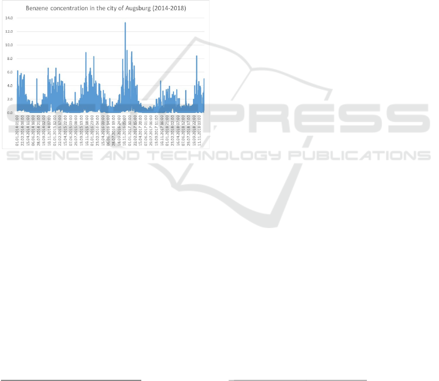
The overall dataset for our study covers the period
between 01.01.2014 and 31.12.2018 with a total of
43,824 hours of data. Traffic data for two major access
roads to the city of Augsburg was provided by the
German Federal Roads Agency (Bundesanstalt für
Benzene Prediction: A Comparative Study of ANFIS, LSTM and MLR
319

Straßenwesen)
1
. These motorways (A8 – Augsburg
Ost and A8 – Augsburg West) use automatic traffic
counting systems to register all vehicles. The benzene
(C
6
H
6
) concentration in the city of Augsburg was
collected from the Bavarian State Office for the
Environment (Bayerisches Landesamt für Umwelt)
2
and is reported in μg/m
3
. Finally, temperature,
precipitation, relative humidity, sunshine duration,
wind speed and wind direction were available from the
German Meteorological Service (Deutscher
Wetterdienst)
3
. As road traffic variable we add up the
vehicles from both roads to get a single traffic
indicator on an hourly basis. Benzene concentration in
Augsburg is used as dependent variable in the
analysis. Figure 1 shows the hourly benzene
concentration in Augsburg between 2014 and 2018.
Figure 1: Hourly benzene concentration in Augsburg,
Germany.
3 METHODS
To assess the forecasting performance for one hour
ahead benzene, multi linear regression, adaptive
neuro-fuzzy inference system and long short-term
memory network are applied and compared. Standard
goodness of fit measures help to evaluate the different
methods and select the best model.
3.1 Multiple Linear Regression
In order to compare the different methods, a multiple
linear regression model (MLR) was estimated as a
base model first. The standard linear regression model
can be described by:
1
https://www.bast.de/BASt_2017/DE/Verkehrstechnik/
Fachthemen/v2-verkehrszaehlung/zaehl_node.html
2
https://www.lfu.bayern.de/luft/immissionsmessungen/
messwertarchiv/index.htm
𝑌=𝛽

+ 𝛽

𝑋

+ 𝛽

𝑋

+⋯+ 𝛽

𝑋

+𝑢 (1)
In that equation Y represents the dependent
variable, β
0
represents the intercept and β
1
is the
parameter related with the first independent variable
X
1
. Further, β
2
is the parameter associated with X
2
and
β
k
is the parameter linked with X
k
. The error term is
labelled u (Wooldridge 2003). The standard multiple
linear regression model implies a linear relationship
among the dependent and the independent variables.
3.2 Adaptive Neuro-Fuzzy Inference
System
The adaptive neuro-fuzzy inference system (ANFIS)
was developed by Jang (1993) and is a combined
model that incorporates a fuzzy system with an
artificial neural network (ANN). The idea here is to
combine the advantages of both methods. The ANFIS
model is defined as a fuzzy inference system (FIS)
with distributed parameters (Quej et al., 2017). In our
analysis a Sugeno first-order fuzzy model is used (for
a discussion see Sugeno, 1985 and Takagi et al.,
1983). In a first-order Sugeno system, a typical rule
has the form:
If input 1 is x and input 2 is y, then output is given by
z = ax + by + c
For a fuzzy inference system with two inputs x and
y as well as one output variable z, with two Sugeno
type fuzzy if-then rules, according to Sugeno (1985)
and Takagi et al. (1983) we get:
Rule 1:
If x is A
1
and y is B
1
, then f
1
= p
1
x + q
1
y + r
1
(2)
Rule 2:
If x is A
2
and y is B
2
, then f
2
= p
2
x + q
2
y + r
2
(3)
In the equations, the parameters in the then-part of
the first-order Sugeno fuzzy model are labelled p
1
, q
1
,
r
1
and p
2
, q
2
, r
2
respectively (Jang 1993).
Following Jang (1993) the ANFIS system contains
five-layers. The first layer is related to a fuzzy model
(Ausati et al. 2016). Each node i in the first layer is a
node function:
𝑂


= 𝜇

(𝑥) (4)
where the parameter x is the input node i, and A
i
is the fuzzy set (linguistic label) associated with this
3
https://opendata.dwd.de/climate_environment/CDC/
observations_germany/climate/hourly/
NCTA 2021 - 13th International Conference on Neural Computation Theory and Applications
320

node function. Thus, 𝑂


is defined by the shape of the
membership function of A
i
and identifies the degree to
which a given value of x fulfils the linguistic label
(Jang, 1993). Typical shapes of membership functions
are triangular, trapezoidal, gaussian or bell-shaped.
They are all bounded between zero and one.
The second layer (product layer) multiplies the
incoming signals and sends out the result.
𝑤

= 𝜇

(
𝑥
)
∗ 𝜇

(
𝑦
)
, 𝑖 = 1,2 (5)
The third layer (normalized layer) calculates the
ratio of the i
th
rule’s strength compared to the sum of
strength of all rules (Jang, 1993 and Quej et al., 2017):
𝑤

=




 

, 𝑖 = 1,2 (6)
In the fourth layer (de-fuzzy layer), the weighted
output of each linear function is derived by:
𝑂


= 𝑤

𝑓

= 𝑤

(𝑝

𝑥+ 𝑞

𝑦+𝑟

(7)
where 𝑤

is the output of the third layer and the
parameter set is given by p
i
, q
i
and r
i
. These parameters
are called consequent parameters (Jang, 1993).
In the fifth layer (total output layer) the overall
output of all incoming signals is calculated as the sum
of all input signals:
𝑂


=
∑
𝑤

𝑓

=
∑




∑


(8)
The figure below shows the ANFIS structure:
Figure 2: ANFIS structure (Guneri et al., 2011).
For the analysis, we apply two triangular
membership functions for every input variable in the
fuzzy inference system. The triangular membership
function can be formulated as follows:
𝜇

(
𝑥
)
=𝑚𝑎𝑥𝑚𝑖𝑛



,



,0 (9)
In this equation the parameters a, b and c change
the shape of the triangular membership function.
Furthermore, the triangular membership function is
bounded between a maximum value of 1 and
minimum value of 0.
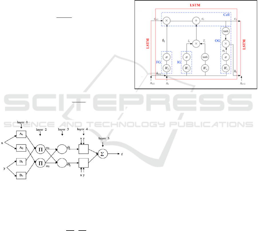
3.3 Long Short-Term Memory Network
The long short-term memory network (LSTM) was
originally introduced by Hochreiter and Schmidhuber
(1997). In contrast to standard recurrent neural
networks (RNN) the LSTM considers both, the short-
term as well as long-term dependency of a time series.
Thus it exhibits temporal dynamic behaviour for a
time sequences (Greff, 2016). The LSTM that is used
in this paper can be found in Fig. 3 and is composed
of cell, input gate, output gate, and forget gate.
Figure 3: LSTM structure (Bai et al., 2019).
The forget gate (FG) determines what information is
removed from the cell state.
𝑓

= 𝜎(𝑊

⋅

ℎ

,𝑥


+𝑏

) (10)
With h
t-1
as the output of the previous cell state and x
t
as the input of the current cell state. The expressions
W
f
and b
f
represent the weights and the bias of the
forget gate respectively, whereas σ refers to the
sigmoid function (Le et al. 2019). The value f
t
is
bounded between 0 (full fail) and 1 (full pass) to
denote the degree of information withholding (Bai,
2019).
The input gate (IG) determines what new
information will be added to the cell state.
𝑖

=𝜎(𝑊

⋅

ℎ

,𝑥


+𝑏

, (11)
𝑐̃

=tanh(𝑊

⋅

ℎ

,𝑥


+𝑏

(12)
and
𝑐

= 𝑓

× 𝑐

+ 𝑖

× 𝑐̃

(13)
With W
i
and b
i
as weights and bias for the input gate,
whereas W
c
and b
c
are the weights and the bias of the
cell state (Le at al. 2019). The operator × stands for
point-wise multiplication. Equations 15 and 16
Benzene Prediction: A Comparative Study of ANFIS, LSTM and MLR
321

calculate the information to be updated, whereas
equation 17 realizes the cell state update (Bai, 2019).
The output gate (OG) controls the current
information in the cell state to flow into the outputs.
𝑜

=𝜎(𝑊

⋅

ℎ

,𝑥


+𝑏

(14)
and
ℎ

=𝑜

× tanh (𝑐

) (15)
With W
o
and b
o
as weights and bias of the output gate.
The term o
t
evaluates which part of the cell state is
exported. The expression h
t
calculates the final output
(Bai, 2017).
3.4 Model Evaluation
In order to achieve the goal of the article, the in- and
out-of-sample forecasting performance of the
different models must be evaluated. To do so, we
apply the means squared error (MSE), the root mean
squared error (RMSE), r-squared (R2) and the mean
absolute error (MAE).
The mean squared error (MSE) is calculated as the
average squared difference between the forecasted
output y and the actual value 𝑦 (Ciaburro, 2017):
𝑀𝑆𝐸 =


(∑
(𝑦

−𝑦

)



)
(16)
Lower values of MSE indicate a better
performance of the model. The square root of the MSE
yields the root mean squared error (RMSE). In
contrast to the MSE, the RMSE measure has the same
units as the forecasted variable. The RMSE is
calculated as:
𝑅𝑀𝑆𝐸 =

∑
(




)




(17)
The mean solute error (MAE) can be calculated by:
𝑀𝐴𝐸 =


∑|
𝑦

−𝑦

|


(18)
The MAE penalizes large and small differences
from the actual by the same amount as the size of the
error, whereas MSE penalizes bigger errors more
(Fenner, 2020).
The coefficient of determination (R
2
) is the ratio
of the explained sum of squares to the total sum of
squares (Studenmund, 2001). The R
2
is bounded
between zero (the variation in the data cannot be
explained at all by the model) and one (the model
perfectly explains the variation in the data). The R
2
is
calculated by:
𝑅

=1−
∑
(




)



∑
(




)



(19)
All four performance measures are used and
compared in order to evaluate the different models.
4 RESULTS
The in-sample period comprises of four years (2014-
2017) and the out-of-sample period of one year
(2018). Therefore, we use 80% of the data as training
set and the remaining 20% as testing set. The table 1
below shows the outcome of the in- and out-of-sample
performance measures of MLR, ANFIS and LSTM in
predicting benzene concentration. For the in-sample
results, the ANFIS method has the highest predictive
power, whereas MLR and LSTM have a very similar
predictive power for one hour ahead benzene
forecasting. However, the out of sample results
indicate that the LSTM has the best forecasting
performance in terms of RMSE, MAE and MSE,
whereas the MLR and ANFIS show similar results.
Only the R
2
is the highest for ANFIS in the out of
sample period.
Table 1: Forecasting benzene one hour ahaead.
MLR ANFIS LSTM
R
2
in sample
0.3767 0.5022 0.3806
RMSE
in sample
0.6617 0.5913 0.6642
MAE
in sample
0.4206 0.3627 0.3906
MSE
in sample
0.4378 0.3496 0.4412
R
2
out of
sample
0.3167 0.3875 0.2727
RMSE
out of
sample
0.5233 0.5272 0.4710
MAE
out of
sample
0.3907 0.3644 0.2814
MSE
out of
sample
0.2738 0.2779 0.2218
NCTA 2021 - 13th International Conference on Neural Computation Theory and Applications
322

5 DISCUSSION
A major advantage of LSTM networks is the ability to
forget part of its previously stored memory and also
add a part of new information to its memory. The
results in this paper support the usefulness of this
unique ability in out of sample forecasting. However,
at least in the used in-sample, LSTM networks could
not outperform ANFIS. Future research should verify
whether this result can be confirmed with other
pollutants and different samples.
Generally, the different methods that were applied
can only explain between 37% and 50% of the
variance in sample and between 27% and 38% out of
sample. Thus a large share of variance cannot be
explained by the models. The inclusion of other
lagged pollutants might help to improve the
forecasting performance. Some authors have extended
the independent variables by other pollutants and
reported an improvement in the forecasting
performance (see inter alias Oprea et al., 2017)).
Moreover, the traffic data could not be collected in the
city centre where the benzene concentration is
measured. As a result, the traffic data from the
highway crossing by the city of Augsburg was used
and this can only serve as an indicator of vehicle
traffic. A precise traffic measurement might therefore
improve benzene predictability.
Furthermore, one hour ahead forecasting is a fairly
short period for traffic emissions and for longer
periods it must be expected that the models become
less predictive. Thus, future research should also
investigate the long term predictability of benzene by
ANFIS, MLR and LSTM. Nonetheless, the results
show that machine learning algorithms in general, and
LSTM in particular might be helpful in predicting
benzene concentration in advance. This can help
traffic management systems to anticipate raising air
pollution and reduce traffic by temporary restrictions.
Not least because of the decision of the European
Court of Justice, it is necessary to immediately reduce
air pollution in German cities. The automatic traffic
counting stations already make it possible to forecast
the development of air pollution. Therefore, the
findings of this article should be used by local
authorities to introduce a traffic control system
promptly and to curb traffic in case of high predicted
air pollution. In addition, it is necessary to install more
traffic counting stations and also the number of air
monitoring stations should be increased to achieve a
more accurate forecast of air pollutants.
6 CONCLUSION
In this paper the predictive power of adaptive neuro-
fuzzy inference systems, long short-term memory
networks and multiple linear regression models for
one hour ahead benzene prediction in the city of
Augsburg is analysed. Artificial intelligence methods
have been used for air pollution forecasting before, but
we add to the literature in benzene prediction and in
the use of long short-term memory networks. The
results of the analysis indicate that adaptive neuro-
fuzzy inference systems have the best in sample
performance for benzene prediction, whereas long
short-term memory networks and multiple linear
regressions show similar predictive power. However,
long short-term memory models have the best out of
sample performance for one hour ahead benzene
prediction. This supports the use of long short-term
memory networks for benzene prediction in real world
applications.
REFERENCES
Ausati, S., Amanollahi, J. (2016). Assessing the accuracy of
ANFIS, EEMD-GRNN, PCR, and MLR models in
predicting PM2.5, Atomspheric Environment, 142, pp.
465-474.
Bai, Y., Zeng, B., Li, C., Zhang, J. (2019). An ensemble
long short-term memory neural network for hourly
PM2.5 concentration forecasting, Chemosphere, Vol.
222, pp. 286-294.
Chang, Y.S., Chiao, H.T., Abimannan, S., Huang, Y.P.,
Tsai, Y.T., Lin, K.M. (2020). An LSTM-based
aggregated model for air pollution forecasting,
Atmospheric Pollution Research, Vol. 11, Issue 8, pp.
1451-1463.
Ciaburro, G. (2017). MATLAB for Machine Learning,
Packt Publishing, Birmingham.
Court of the European Union (2021). Between 2010 and
2016, Germany systematically and persistently
exceeded the limit values for nitrogen dioxide (NO2).
PRESS RELEASE No 94/21, Luxembourg, 3 June
2021, Judgment in Case C-635/18, Commission v
Germany
De Donno, A., De Giorgi, M., Bagordo, F., Grassi, T., Idolo,
Al, Serio, F., Ceretti, E., Feretti, D., Villarini, M.,
Moretti, M., Carducci, A., Verani, M., Bonetta, S.,
Pignata, C., Bonizzoni, S., Bonetti, A., Gelatti, U.
(2018). MAPEC_LIFE Study Group, “Health Risk
Associated with Exposure to PM10 and Benzene in
Three Italian Towns”, International journal of
environmental research and public health, 15(8), 1672.
https://doi.org/10.3390/ijerph15081672
European Environment Agency, (2019). Air quality in
Europe – 2019 report, No 10/2019, ISSN 1977-8449.
Benzene Prediction: A Comparative Study of ANFIS, LSTM and MLR
323

European Environment Ageny, (2020). Health impacts of air
pollution, last modified 28 Jan 2020, https://www.eea.
europa.eu/themes/air/health-impacts-of-air-pollution
Fenner, M.E. (2020). Machine Learning with Python for
Everyone, Pearson Education Inc.
German Federal Environment Agency (2021). Benzene is an
organic, chemical compound with an aromatic odour. It
is carcinogenic and a content of petrol.
https://www.umweltbundesamt.de/en/topics/air/air-
pollutants-at-a-glance/benzene#emission-sources
Greff, K., Srivastava, R.K., Koutník, J., Steunebrink, B.,
Schmidhuber, J. (2016). LSTM: a search space odyssey,
IEEE Trans. Neural Netw. Learn. Syst., 28 (10), pp.
2222-2232.
Guneri, A.F., Ertay, T., Yücel, Y. (2011). An approach
based on ANFIS input selection and modeling for
supplier selection problem, Expert Systems with
Applications, 38, 14907-14917.
Hochreiter, S., Schmidhuber, J. (1997). Long Short-term
Memory. Neural Computation, 9 (8): 1735-80.
DOI:10.1162/neco.1997.9.8.1735.
Humpe, A., Brehm, L., Günzel, H. (2021). Forecasting Air
Pollution in Munich: A Comparison of MLR, ANFIS,
and SVM, in Proceedings of the 13th International
Conference on Agents and Artificial Intelligence -
Volume 2: ICAART, ISBN 978-989-758-484-8, pages
500-506. DOI: 10.5220/0010184905000506
Jang, J.S.R. (1993). ANFIS: adaptive-network-based fuzzy
inference system, IEEE Transactions on Systems, Man,
and Cybernetics, 23 (3), 665-685, doi: 10.1109/
21.256541.
Karakitsios, S.P., Papaloukas, C.L., Kassomenos, P.A.,
Pilidis, G.A. (2006). Assestment and prediction of
benzene concentration in a street canyon using artificial
neural networks and deterministic models. Their
response to “what if” scenarios”, Ecological Modelling,
193, pp. 253-270.
Kaur M., Mandal, A. (2020). PM2.5 Concentration
Forecasting using Neural Networks for Hotspots of Delhi,
International Conference on Contemporary Computing
and Applications (IC3A), Lucknow, India, 2020, pp. 40-
43, doi: 10.1109/IC3A48958.2020.233265.
Krzyzanowski, M., Kuna-Dibbert, B., Schneider, J. (2005).
Health effects of transport-related air pollution, WHO
Library Cataloguing in Publication Data, ISBN 91-890-
1373-7.
Künzli, N., Kaiser, R., Medina, S., Studnicka, M., Chanel,
O., Filliger, P., Herry, M., Jr. Horak, F., Puybonnieux-
Texier, V., Quénel, P., Schneider, J., Seethaler, R.,
Vergnaud, J.C., Sommer, H. (2000) Public-health
impact of outdoor and traffic-related air pollution: a
European assessment, Lancet, 356(9232), 795-801. doi:
10.1016/S0140-6736(00)02653-2, PMID: 11022926.
Le X-H, Ho HV, Lee G, Jung S. (2019). Application of Long
Short-Term Memory (LSTM) Neural Network for Flood
Forecasting. Water 11(7): 1387. https://doi.org/10.3390/
w11071387
Lee, C.Y., Lee, Z.J., Huang, J.Q., Ye, F.L., Ning, Z.Y.,
Yang, C.F. (2019). Urban Air Quality Analysis and
Forecast Based on Intelligent Algorithm with Parameter
Optimization and Decision Rules, Applied Sciences, 9,
5445.
Loya, N., Pineda, I.O., Pinto, D., Gomez-Adorno, H.,
Aleman, Y. (2012). Forecast of Air Quality Based on
Ozone by Decision Trees and Neural Networks,
Mexican International Conference on Artificial
Intelligence (MICAI), in: I. Batyrshin, M. González
Mendoza (eds) Advances in Artificial Intelligence,
MICAI 2012, Lecture Notes in Computer Science, 2013,
vol 7629, pp. 97-106, Springer, Berlin, Heidelberg.
https://doi.org/10.1007/978-3-642-37807-2_9
Ly, H.B., Le, L.H., Phi, L.V., Phan, V.H., Tran, V.Q., Pham,
B.T., Le, T.T., Derrible, S. (2019). Development of an
AI Model to Measure Trafic Air Pollution from
Multisensor and Weather Data, Sensors, 19 (22), 4941,
DOI: 10.3390/s19224941
Mihalache, S.F., Popescu, M. (2016). Development of
ANFIS Models for PM Short-term Prediction, Case
Study, 8th International Conference on Electronics,
Computers and Artificial Intelligence (ECAI), Ploiesti,
pp. 1-6, doi: 10.1109/ECAI.2016.7861073.
Molina-Cabello, M.A., Passow, B., Domínguez, E.,
Elizondo, D., Obszynska, J. (2019). Infering Air Quality
from Traffic Data Using Transferable Neural Network
Models, in: Advances in Computational Intelligence,
15th International Work-Conference on Artificial
Neural Networks, IWANN 2019, Gran Canaria, Spain,
June 12-14, 2019, Proceedings, Part I, pp.832-843, DOI:
10.1007/978-3-030-20521-8_68.
Oprea M., Popescu, M., Mihalache, S., Dragomir, E. (2017).
Data Mining and ANFIS Application to Particulate
Matter Air Pollutant Prediction. A Comparative Study,
in Proceedings of the 9th International Conference on
Agents and Artificial Intelligence, Volume 1: ICAART,
ISBN 978-989-758-220-2, pages 551-558. DOI:
10.5220/0006196405510558
Pawlak, I., Jaroslawski, J. (2019). Forecasting of Surface
Ozone Concentration by Using Artificial Neural
Networks in Rural and Urban Areas in Central Poland,
Atmosphere, 10, 52.
Quej, V.H., Almorox, J., Arnaldo, J.A., Saito, L., (2017).
ANFIS, SVM and ANN soft-computing techniques to
estimate daily global solar radiation in a warm sub-
humid environment, Journal of Atmospheric and Solar-
Terrestrial Physics, Volume 155, Pages 62-70,
https://doi.org/10.1016/j.jastp.2017.02.002.
Sayeed, A., Choi, Y., Eslami, E., Lops, Y., Roy, A., Jung, J.
(2020). Using a deep convolutional neural network to
predict 2017 ozone concentrations, 24 hours in advance,
Neural Networks, Vol. 121, pp. 396-408.
Smith, M.T. (2010). Advances in understanding benzene
health effects and susceptibility, Annu. Rev. Public
Health, 31:133–148. doi: 10.1146/annurev.publ
health.012809.103646.
Studenmund, A.H., (2001). Using Econometrics: A practical
guide, Addison Wesley Longman Inc.
Sugeno, M., (1985). Industrial Applications of Fuzzy Control,
Elsevier Science Inc., ISBN: 978-0-444-87829-8
Takagi, T., Sugeno, M. (1983). Derivation of fuzzy control
rules from human operator’s control actions, Proc IFAC
NCTA 2021 - 13th International Conference on Neural Computation Theory and Applications
324

Symp. Fuzzy Inform., Knowledge Representation and
Decision Analysis, pp. 55-60.
The Lancet Commission, (2017). The Lancet Commission
on Pollution and Health, Lancet, doi: 10.1016/S0140-
6736(17)32345-0.
Wooldridge, J.M. (2003). Introductory Econometrics: A
Modern Approach, 2e, Thomson, South-Western, p. 71.
Benzene Prediction: A Comparative Study of ANFIS, LSTM and MLR
325