Specialized Neural Network Pruning for Boolean Abstractions
Jarren Briscoe
1,2 a
, Brian Rague
1 b
, Kyle Feuz
1 c
and Robert Ball
1 d
1
Department of Computer Science, Weber State University, Ogden, Utah, U.S.A.
2
Department of Computer Science, Washington State University, Pullman, Washington, U.S.A.
Keywords:
Neural Networks, Network Pruning, Boolean Abstraction, Explainable AI, XAI, Interpretability.
Abstract:
The inherent intricate topology of a neural network (NN) decreases our understanding of its function and
purpose. Neural network abstraction and analysis techniques are designed to increase the comprehensibility
of these computing structures. To achieve a more concise and interpretable representation of a NN as a
Boolean graph (BG), we introduce the Neural Constantness Heuristic (NCH), Neural Constant Propagation
(NCP), shared logic, the Neural Real-Valued Constantness Heuristic (NRVCH), and negligible neural nodes.
These techniques reduce a neural layer’s input space and the number of nodes for a problem in NP (reducing
its complexity). Additionally, we contrast two parsing methods that translate NNs to BGs: reverse traversal
(N ) and forward traversal (F ). For most use cases, the combination of NRVCH, NCP, and N is the best
choice.
1 INTRODUCTION
1.1 Background
While NNs are a powerful machine learning tool, they
are semantically labyrinthine. The most essential at-
tribute lacking in the interpretability of NNs is con-
ciseness (Briscoe, 2021). This explains why many
authors have opted to use Boolean graphs (BGs) as an
explanatory medium (Briscoe, 2021; Brudermueller
et al., 2020; Shi et al., 2020; Choi et al., 2017; Chan
and Darwiche, 2012). However, this problem is in NP,
and we introduce heuristics and traversal methods to
reduce the complexity.
Neural Networks. Neural networks train on a data
set containing inputs and classifications (supervised
learning), unlabelled data (unsupervised learning), or
policies (reinforcement learning). After training, the
neural network predicts classifications for new inputs.
Since neural network structures and algorithms are
quite diverse, in this paper we limit the scope of neural
networks to the most common type. Specifically, they
are acyclic, symmetric, first-order neural networks
a
https://orcid.org/0000-0002-7422-9575
b
https://orcid.org/0000-0001-9065-6780
c
https://orcid.org/0000-0003-3730-3198
d
https://orcid.org/0000-0001-5302-5293
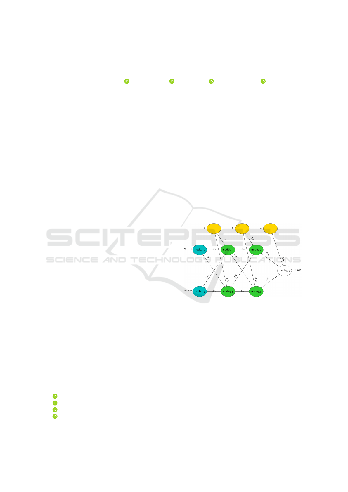
Figure 1: A multilayer perceptron. The hidden nodes
(node
1,0
, node
1,1
, node
2,0
, and node
2,1
) and the output node
(node
3,0
) use the σ activation function. The legend’s re-
mainder is as follows: the input nodes are in the leftmost
layer (node
0,0
and node
0,1
) and the bias nodes are in the top
row (unlabeled).
with a finite amount of layers and nodes with binary
input and real-valued activations (e.g., a multilayer
perceptron such as Figure 1) or an autoencoder). For
formal definitions of neural networks, see Neural Net-
work Formalization (Fiesler, 1992).
Explaining Neural Networks. From the many
techniques attempting to conceptualize and explain
neural networks (Guidotti et al., 2018; Andrews et al.,
1995; Baehrens et al., 2010; Brudermueller et al.,
2020; Shi et al., 2020; Choi et al., 2017; Briscoe,
2021), three generic categories emerge: decomposi-
178
Briscoe, J., Rague, B., Feuz, K. and Ball, R.
Specialized Neural Network Pruning for Boolean Abstractions.
DOI: 10.5220/0010657800003064
In Proceedings of the 13th International Joint Conference on Knowledge Discovery, Knowledge Engineering and Knowledge Management (IC3K 2021) - Volume 2: KEOD, pages 178-185
ISBN: 978-989-758-533-3; ISSN: 2184-3228
Copyright
c
 2021 by SCITEPRESS – Science and Technology Publications, Lda. All rights reserved

tional, eclectic, and pedagogical.
Decompositional techniques consider individual
weights, activation functions, and the finer details of
the network (local learning). For example, abstracting
each node of the NN with its weights is a decomposi-
tional technique.
On the other hand, a pedagogical approach dis-
covers through an oracle or teacher (global learn-
ing). This approach allows underlying machine learn-
ing structure(s) to be versatile—this technique will
remain viable if the neural network black-box is re-
placed with a support-vector machine (SVM). A sim-
ple example of a pedagogical representation is a deci-
sion tree whose training inputs are fed into a NN, and
the decision tree’s learned class values are the output
of the NN.
Finally, eclectic approaches combine the decom-
positional and pedagogical techniques. An example
of an eclectic approach is directing a learning algo-
rithm over neural nodes (decompositional and local)
while determining and omitting inputs negligible to
the final result (pedagogical and global).
This work introduces node reduction techniques
and contrasts two neural network traversal methods
to translate neural networks to the more interpretable
and formally verifiable BGs. The forward traversal,
F is strictly decompositional while the reverse traver-
sal, N , is mostly decompositional with some peda-
gogical aspects (eclectic).
1.2 Format
This paper is organized as follows: Section 2 articu-
lates our motivation, Section 3 surveys related work;
Section 4 generalizes allowable activation functions
and thresholds for the heuristics and traversal algo-
rithms introduced; Section 5 defines our symbols and
data structures; Section 6 explains our heuristics and
their cascading effects; Section 7 defines the network
traversals N and F ; finally, Section 8 gives a sum-
mary and addresses future work.
2 MOTIVATION
2.1 Overview
This intrinsic incoherent nature of NNs has inhibited
the widespread adoption of these computational struc-
tures primarily due to the lack of accountability (Kroll
et al., 2016), liability (Kingston, 2016), and safety
(Danks and London, 2017) when applied to sensitive
tasks such as predicting qualified job candidates and
medical treatments.
Figure 2: A type of BG, a binary decision diagram (BDD),
that represents a neural network. [L0X0, L0X1, L0X2,
L0X3] 7→ [marginal adhesion, clump thickness, bare nuclei,
uniformity of cell shape].
Furthermore, some legal guidelines distinctly pro-
hibit black-box decisions to prevent potential discrim-
ination (such as Recital 71 EU DGPR of the EU gen-
eral data protection regulation). Additionally, safety-
critical applications have avoided neural networks be-
cause of their inaccessibility to feasible formal ver-
ification techniques. For example, neural-network-
driven medical devices or intrusion prevention sys-
tems on networks required to maintain accessibility
(such as military communication) lack formal veri-
fication and have serious risks. This work helps all
of these avenues by reducing the computational com-
plexity to approximate neural networks.
2.2 Example
Consider a neural network that classifies a tumor as
benign or cancerous. Medical practitioners would
benefit from understanding the logic behind the NN
to diagnose tumors without using the NN, to explain
them to patients, and to investigate the causes of the
logic. Humans cannot simply understand the NN. To
compensate, a general algorithm that transforms NNs
to BGs, B, assists human comprehension.
Let this cancer/benign classifier have binary and
ordered inputs [marginal adhesion, clump thickness,
bare nuclei, uniformity of cell shape]. To binarize
the data, a single pivot is used as these inputs main-
tain significance with a single bit. However, mul-
tiple bits may be needed for nonlinear correlations.
Using the ideas in this paper, a BG is extracted
such as Figure 2 (illustrated with ABC (Brayton and
Mishchenko, 2010)). From this BG, the medical prac-
titioner can understand the logic, investigate it, and
explain it to patients as needed.
3 STATE OF THE ART
The simplest and least efficient method to approx-
imate neural nodes is the brute-force method with
Θ(2
n
n) complexity where n is the number of in-
degree weights for a given node. Fortunately, there
Specialized Neural Network Pruning for Boolean Abstractions
179

are several far more efficient methods. The expo-
nentially upper-bound methods described below yield
higher accuracy than the pseudo-polynomial methods
that follow. We denote a generic NN to BG algorithm
as B.
Exponential Methods. An exponential method tar-
geting Bayesian network classifiers reports a com-
plexity of O(2
0.5n
n) (Chan and Darwiche, 2012).
While this approximation was done for Bayesian net-
work classifiers, the correlation to neural node ap-
proximation can be formalized (Choi et al., 2017).
Another algorithm to approximate neural nodes ex-
hibits a complexity of O(2
n
) (Briscoe, 2021).
Current Work. N improves the upper-bound ex-
ponential complexity of Chan and Darwhiche’s algo-
rithm as applied to neural networks (Choi et al., 2017)
with no loss in accuracy. Assuming a ratio x : T of
constant nodes to the total number of nodes, the new
complexity becomes O(2
0.5n(1−x)
n).
Pseudo-Polynomial Methods Faster methods that
compute a neural node with less accuracy produce a
pseudo-polynomial O(n
2
W )
1
complexity where
W = |θ
D
| +
∑
w∈node
i, j
|w|. (1)
θ
D
is the threshold in the activation function’s do-
main, and node
i, j
is a vector of in-degree weights.
Furthermore, these weights must be integers with
fixed precision (Shi et al., 2020).
If one uses a constant maximum depth d for the
binary decision tree (Briscoe, 2021), then the entire
neural network can be computed in O(n) time where
n is the number of neural nodes. This is a pseudo-
polynomial complexity since the constant d causes
the individual neural node approximation to be a con-
stant of O(2
d
) = O(1) and is still O(2
n
) for n < d.
Of course, if d is not constant, then the neural node
complexity becomes O(2
min(n,d)
).
We are currently working on creating a flexible
maximum depth that considers the weight vector’s
distribution and size. Future work could extend this
idea to Chan and Darwhiche’s algorithm on Bayesian
Network classifiers and reduce the O(2
0.5n
n) com-
plexity with minimal accuracy loss (and as employed
by (Choi et al., 2017)). Enforcing a maximum
depth is equivalent to capping a maximum amount
1
While the original text only mentions the O(nW ) com-
plexity to compile the OBDD (Shi et al., 2020), the com-
plexity to approximate the node is O(n
2
W ).
of weights considered, and since the weights’ im-
portance are ordered by the greatest absolute value
(Briscoe, 2021), the weights with the smallest abso-
lute values should be omitted first.
Final Product. The NN can be mapped to any
Boolean structure. Shi et al. and Choi et al. used
Ordered Binary Decision Diagrams (OBDDs) and
Sentential Decision Diagrams (SDDs) while Bruder-
mueller et al. and Briscoe employed And-Inverter
Graphs (AIGs) (Shi et al., 2020; Choi et al., 2017;
Briscoe, 2021; Brudermueller et al., 2020). However,
other Boolean structures exist with different topolog-
ical and/or operational features that highlight specific
design (e.g. comprehensibility, Boolean optimiza-
tions, and hardware optimizations). The final product
for this work is abstracted as a BG (Boolean Graph)
and illustrated with ABC (Brayton and Mishchenko,
2010).
Neural Pruning. While traditional neural pruning
methods seek to reduce overfitting, speedup neu-
ral networks, or even improve accuracy (Han et al.,
2015), our pruning algorithm is specialized for inter-
pretability and to reduce the worst-case complexity of
B. So our network pruning is not directly comparable
to traditional pruning to the best of our knowledge.
4 ACTIVATION FUNCTIONS
Shi and Choi only considered ReLU and sigmoid
functions (Shi et al., 2020; Choi et al., 2017). We
extend the allowed activation functions to any that
allow a reasonable Boolean cast (Conjunctive Limit
Constraint) and conversion to a binary step function
(Diagonal Quadrants Property).
Conjunctive Limit Constraint.
lim
θ→−∞
f (θ) = 0 and lim
θ→∞
f (θ) > 0 (2)
The conjunctive limit constraint allows us to treat
one side of the range threshold as false (analogous
to zero) and the other side as true (analogous to a
positive number). Functions that have negative and
positive limits (such as tanh) are better defined within
an inhibitory/excitatory context. It can be experimen-
tally shown that the accuracy for NN to BG methods
decreases for functions like tanh. The Swish acti-
vation function (Ramachandran et al., 2017) lies in
between the inhibitory/excitatory and true/false spec-
trums since there are negative range values but it still
satisfies the Conjunctive Limit Constraint.
KEOD 2021 - 13th International Conference on Knowledge Engineering and Ontology Development
180

Diagonal Quadrants Property. Converting a real-
valued function ( f
R
) to a binary-step function ( f
B
)
is best suited for real-valued functions that only lie
in two diagonal quadrants or on the boundaries, cen-
tered on the threshold f
R
(θ
D
) = θ
R
. Consider the
sigmoid function σ
R
(θ) =
1
1+e
−θ
. Since σ
R
’s range
(R ) is in (0,1), we want the range’s threshold, θ
R
, to
be 0.5 which corresponds to θ
D
= 0 on the domain:
σ
R
(0) = 0.5. Drawing horizontal and vertical lines
through σ
R
(0) = 0.5 creates the quadrants. Since σ
R
with threshold σ
R
(0) = 0.5 is contained in diagonal
quadrants (top-right and bottom-left—see Figure 3),
this activation function is suitable for conversion to a
binary-step function σ
B
. With the threshold θ
R
:
σ
B
(θ;σ
R
,θ
R
) =
(
1 if σ
R
(θ) ≥ θ
R
,
0 otherwise.
(3)
For monotonic functions, any threshold satisfies
the diagonal quadrant property. However, a reason-
able threshold choice increases the accuracy of the
conversion algorithm—if one chooses the threshold
σ
R
(−10000) ≈ 0 then the BG will almost certainly
always yield true.
Threshold on the Domain (θ
D
). Since this work is
limited to activation functions satisfying the Diago-
nal Quadrant Property, the threshold can be uniquely
identified by only considering the domain. Once the
domain’s threshold is found, the activation function
and range threshold can be effectively discarded. The
more computationally efficient (and equivalent) defi-
nition of σ
B
is then:
σ
B
(θ;θ
D
) =
(
1 if θ ≥ θ
D
,
0 otherwise.
2
(4)
Henceforth, θ
D
= 0 and when σ
B
is used without
all parameters, the implicit parameters are (θ;0).
5 DATA STRUCTURE
5.1 Neural Network Data Structure
The neural network, NN, is defined as an array of lay-
ers.
NN ← [l
1
,l
2
,.. .,l
m
] (5)
2
Since σ
B
(θ
D
) is undefined, letting σ
B
(θ
D
) = 0 or
σ
B
(θ
D
) = 1 is arbitrary or dependent on special cases.
Figure 3: σ
R
(θ) with a threshold of σ
R
(0) = 0.5 satisfies
the diagonal quadrants property.
Each layer, l
i
, is an array of nodes.
l
i
← [node
i,0
,node
i,1
,.. .,node
i,n
] (6)
Each node
i, j
is an array of in-degree weights where
w
i, j,b
is the bias weight and w
i, j,k
is the weight from
node
i−1,k
to node
i, j
.
node
i, j
← [w
i, j,b
,w
i, j,0
,w
i, j,1
,.. .,w
i, j,p
] (7)
In the context of the current node
i, j
, the bias
weight is expressed as: b = w
i, j,b
.
Output Definitions. out
i
is the array of binarized
outputs for layer l
i
and o
i, j
is the binarized output of
node
i, j
.
out
i
← [o
i,0
,o
i,1
,.. .,o
i,n
] (8)
Since the neural network uses the σ
R
activation
function (Figure 3), we use the σ
B
binary-step func-
tion as defined in Section 4 with the threshold θ
D
= 0.
Note that the θ in activation functions f (θ) is actually
a dependent variable:
θ = θ(~x,~w,b) =~x ·~w + b. (9)
The inputs ~x = out
i−1
, the weights ~w = node
i, j
\
w
i, j,b
, and the bias b = w
i, j,b
.
o
i, j
= σ
B
(θ(out
i−1
,node
i, j
\ b, b)) =
(
1 if θ ≥ 0,
0 otherwise.
(10)
The first layer, l
0
, has no in-degree weights and
out
0
is the binary inputs for the neural network.
Specialized Neural Network Pruning for Boolean Abstractions
181

6 HEURISTICS AND
PROPAGATION
6.1 Neural Constantness Heuristic
(NCH)
The Neural Constantness Heuristic (NCH) checks for
a neural node’s constantness with exactly linear com-
putational complexity where n is the number of in-
degree weights for a given node. To understand this
heuristic, let us create some variables and functions.
For node
i, j
:
• Let b be the bias weight w
i, j,b
.
• Let W
+
be the set of weights greater than zero in
node
i, j
\ b
• Let GV
i, j
be the largest possible combination of
weights in node
i, j
.
GV
i, j
= b +
∑
w∈W
+
w (11)
• Let W
−
be the set of weights less than zero in
node
i, j
\ b.
• Let SV
i, j
be the smallest possible combination of
weights in node
i, j
.
SV
i, j
= b +
∑
w∈W
−
w (12)
As seen above, b is always true and must be consid-
ered when computing both GV
i, j
and SV
i, j
regardless
of its positivity. A heuristic to find the binarized out-
put for a neural node is then:
o
i, j
←





1 if SV
i, j
≥ 0,
0 if GV
i, j
≤ 0
B otherwise.
(13)
The logic is if the greatest possible value of θ is
less than zero, then B will produce a constant false.
Alternatively, if the smallest possible value is greater
than zero B yields true. Otherwise, B approximates
the node.
6.2 Neural Real-valued Constant
Heuristic (NRVCH)
Here, we extend NCH to approximate nodes as real-
valued instead of binary. The Neural Real-Valued
Constant Heuristic (NRVCH) has less than or equal to
B with NCH’s sum-squared error. Furthermore, we
find that NRVCH elicits many more constant nodes
than NCH. Since NRVCH assumes an input space in
{0,1}
n
, it must use N . In addition to making the
same assumptions as NCH in Section 6.1, NRVCH
assumes the activation function is monotonically non-
decreasing (as most activation functions are). We as-
sume f = σ; however, NRVCH can be extended to
other functions.
To determine if a node should be approximated as
constant, NRVCH considers a maximum threshold on
the range, α
R
. Then the difference between range ex-
tremes of the weights in node
i, j
are tested to be less
than or equal to α
R
where α
R
≤ 0.5. If the condition
is satisfied, the entire node is estimated as f (avg
D
)
where avg
D
is the average of all 2
n
possible combina-
tions of weights.
NRVCH: o
i, j
←





f (avg
D
)
if f (GV
i, j
) − f (SV
i, j
) ≤ α
R
B otherwise.
(14)
We know that f (LV
i, j
) and f (GV
i, j
) yield the
range extrema of f given node
i, j
since f is monotonic.
Average on the Domain (avg
D
). avg
D
is chosen to
sufficiently approximate the average over the range,
avg
R
, in linear time and to minimize the sum-squared
error (SSE).
For α
R
= 0.5, the worst difference between avg
R
and f (avg
D
) occurs with a weight vector [0,0.5] given
f = σ. Here, σ(avg
D
) = 0.5621 and avg
R
= 0.5612.
While avg
R
gives less error than f (avg
D
), finding
avg
R
is in O(w2
w
) where w is the number of weights.
In contrast, we obtain avg
D
(linear to the number of
weights) by realizing that the power set of {0,1} al-
ways contains equal zeros and ones for each variable
(see Table 1). Because of this, we can sum each
weight, divide the summation by two, and then add
the aggregated bias. Even when previous nodes are
deemed constant and aggregated into the bias, node
i, j
is always in {0, 1}
n
. Substituting this formula for
avg
D
,
o
i, j
←













f



w
i, j,b
+
∑
w∈node
i, j
w
2



if f (GV
i, j
) − f (SV
i, j
) ≤ α
R
B otherwise.
(15)
Theorem 1. avg
R
≈ f (avg
D
) minimizes the sum-
squared error (SSE).
KEOD 2021 - 13th International Conference on Knowledge Engineering and Ontology Development
182

Table 1: The second Cartesian power of {0,1}

{0,1}
2

.
Notice that 0 and 1 are evenly distributed among each vari-
able x
i
.
x
0
x
1
0 0
0 1
1 0
1 1
Proof. SSE is given by
E =
n
∑
i=0
(x
i
− avg
R
)
2
(16)
Where [x
0
,x
1
,.. .,x
n
] is the set of possible activation
outputs.
δE
δavg
R
= −2
n
∑
i=0
(x
i
− avg
R
) (17)
δE
δavg
R
= 0 =
n
∑
i=0
x
i
−
n
∑
i=0
avg
R
(18)
n
∑
i=0
x
i
=
n
∑
i=0
avg
R
= n × avg
R
(19)
avg
R
=
∑
n
i=0
x
i
n
(20)
So avg
R
gives the minimum of E.
Additionally, given α
R
≤ 0.5 and f = σ, NRVCH
has less sum-squared error than NCH and creates con-
stant node approximations at least as often as NCH.
6.3 Neural Constant Propagation
The constantness of previous nodes propagates
throughout the network. While F can inherently in-
tegrate this propagation, N must take a preliminary
forward traversal in linear time. We call this propaga-
tion of constants Neural Constant Propagation (NCP).
Propagation is done by aggregating constant
nodes into the subsequent layer’s bias vector. As such,
some nodes become constant that would not without
NCP. For NCH, the constant nodes may only be rep-
resented as a 0 or 1, whereas NRVCH constants are in
(0,1).
Constant Aggregation Example using NRVCH.
Here, we give an example of a node that is only
constant by NCP. Assume l
i
has real-valued constant
nodes o
i,1
= 0.7 and o
i,2
= 0.5. Then if node
i+1,0
is
[−1,0,3.2, 1] where –1 is the bias weight,
node
i+1,0
← [1.74, 0] since (21)
[1.74,0] = [−1 + 0.7 × 3.2 + 0.5 × 1, 0] (22)
Now, SV
i, j
≥ 0 therefore σ
R
(SV
i, j
) ≥ 0.5. For σ
R
,
f (GV
i, j
) must be less than 1 so
f (GV
i, j
) − f (SV
i, j
) ≤ 0.5 = α
R
. (23)
node
i+1,0
is now constant and will propagate to the
next bias vector. Also, node
i+1,0
is now skipped in N
along with nodes node
i,1
and node
i,3
.
7 NETWORK TRAVERSALS
In this section, we contrast two traversal algorithms:
the forward traversal (F ) and the reverse traversal
(N ).
N discovers and skips negligible neural nodes en-
tirely and ceases parsing at the input layer or upon
finding a negligible layer. Both traversals benefit by
the Neural Constant Propagation (NCP) that consid-
ers the previous layer’s constant nodes (Section 6.3).
However, F benefits more from NCP since F finds
more constant nodes due to entirely approximating
l
i−1
. To benefit from NCP, N employs a preliminary
forward traversal in linear time to find many of the
constant nodes.
With NCP, N improves average complexities for
layers whose input space has a ratio of x : T (num-
ber of constant nodes : total number of nodes) from
O(2
0.5n
n) to O(2
0.5n(1−x)
n) where 0 ≤ 1−x ≤ 1. Sim-
ilarly, F can also reduce the time complexity by omit-
ting weights—however, the NN to BG algorithms
mentioned in this paper cannot take full advantage of
F ’s weight pruning.
7.1 F : Forward Traversal
F approximates each node as a Boolean function one
layer at a time from the input to the output layer.
In contrast to N , F has a finer understanding of
the current layer’s input space (l
i
) since the previous
layer (l
i−1
) has been approximated. We call this type
of knowledge shared logic.
For example, approximating node
3,0
(from Fig-
ure 1) without any reduction has 2
n
inputs (see Ta-
ble 2). However, applying F to Figure 1 up to node
3,0
finds that o
2,0
= o
2,1
. Therefore, the input space for
l
3
is reduced by half to {[0,0], [1,1]} since [0,1] and
[1,0] can never occur. Applying B to the reduced in-
put space, we find that o
3,0
= 1. See the reduced space
in Table 3.
This technique can be extended to greater com-
plexities. For example, if out
2
= [o
2,0
,o
2,1
,o
2,2
] and
F deduces that o
2,0
= o
2,1
+o
2,2
, then the input space
for l
3
can be reduced from 2
3
to 2
2
by removing the
Specialized Neural Network Pruning for Boolean Abstractions
183

Table 2: Exhaustive traversal space for node
3,0
.
o
2,0
o
2,1
θ o
3,0
0 0 1 1
0 1 2 1
1 0 1.1 1
1 1 2.1 1
Table 3: The reduced input space for node
3,0
using F ’s
shared logic.
o
2,0
o
2,1
θ o
3,0
0 0 1 1
1 1 2.1 1
four impossible instances: [1, 0, 0],[0, 1, 1],[0, 1, 0],
and [0,0,1].
Note that the reduced input space does not always
yield an equivalent expression as shown above. The
input space is reduced by asserting logical statements
over primitive inputs (e.g. o
2,0
= o
2,1
+ o
2,2
). This
maintains or reduces the number of true outputs in
the Lookup table (LUT) which may alter the Boolean
logic. However, the logic is effectively the same con-
sidering that only the impossible relations were omit-
ted.
Shared-logic Setbacks. The shared logic advan-
tage of F has three notable setbacks. First, finding the
shared logic may exhibit diminishing returns. Second,
while reducing the available input space can yield
simpler Boolean approximations, post-hoc Boolean
simplification can achieve the same result. Third, the
logic table may be shortened, but the instances of B
mentioned in this paper do not inherently take advan-
tage of input spaces not in {0,1}
n
. Future work can
solve, mitigate, and/or balance these setbacks.
7.2 N : Reverse Traversal
N (see Algorithm 1) does NCP in a single forward
traversal using the heuristics NCH or NRVCH in lin-
ear time. Afterward, N finds more negligible nodes
and approximates the NN in its reverse traversal. This
is done by establishing which outputs, out
i−1
are used
in each node
i, j
∈ l
i
. If no nodes in the previous layer
are used, they are deemed negligible and remembered
in the DoPrevInputsMatter data structure.
Shared Logic. Detecting shared logic to the extent
of F without approximating the entire node (thus de-
feating the purpose for N ) is left for future work.
Algorithm 1: N : Reverse traversal. Here, B integrates the
heuristics (e.g. NRVCH).
Input:
• NN = [l
1
,l
2
,.. .,l
m
].
• θ
D
: the threshold on the domain.
Output: NNBG: a BG approximation of the
neural network.
ct.out = [out
0
, out
1
,.. ., out
i−1
,.. .,out
m−1
] ←
reduced l
i
input spaces using NCP;
ct.bias ← aggregated biases from NCP via
summation;
/* Each node in the final layer
always matters. */
DoCurrentInputsMatter ← [true
0
, true
1
,.. .,
true
length(l
m
)
];
for l
i
← l
m
,l
m−1
,.. .,l
1
do
inputSpace ← ct.out
i−1
;
forall node
i, j
∈ l
i
do
if DoCurrentInputsMatter[ j] then
DoPrevInputsMatter, o
i, j
←
B(node
i, j
,θ
D
,ct.bias
i, j
,inputSpace);
LayerBG
i
← o
i,0
|o
i,1
|.. .|o
i,n
;
if true is not in DoPrevInputsMatter then
break;
DoCurrentInputsMatter ←
DoPrevInputsMatter;
NNBG ← aggregate layers sequentially;
return NNBG
7.3 Traversal Comparison
Let’s compare F and N with the neural network in
Figure 1. Here, N only parses the output node with
three weights while F parses all hidden nodes and the
output node for a total of fifteen weights. N creates
a more concise BG than F since F recalls negligi-
ble node logic. Both traversals implement a Boolean
simplification algorithm after parsing before transla-
tion to a BG.
8 CONCLUSION AND FUTURE
WORK
8.1 Summary
We successfully introduce heuristics (Section 6) and
two traversal techniques (Section 7) the Neural Con-
stant Heuristic (NCH), the Neural Real-Valued Con-
KEOD 2021 - 13th International Conference on Knowledge Engineering and Ontology Development
184

stant Heuristic (NRVCH), the Neural Constant Prop-
agation (NCP), the forward traversal (F ), and the re-
verse traversal (N ).
NCH is functionally equivalent to B (a generic
NN to BG algorithm). NRVCH produces results dif-
ferent from B and produces at most as much sum-
squared error as NCH. Furthermore, NRVCH trans-
lates at least as many nodes to constant values as
NCH. Both heuristics allow some nodes to be calcu-
lated in linear time.
NCP uses constant nodes from previous layers to
reduce the weight space in the current layer. The
propagation technique is better implemented with
NRVCH but can be done with NCH.
F uses its perfect knowledge of the previous layer
to reduce the current layer’s input space via shared
logic and does not complement most B algorithms.
In contrast, N suits many B options and omits neural
nodes or layers entirely.
All things considered, the union of NRVCH, NCP,
and N is often the best choice for computational com-
plexity, conciseness, and accuracy.
8.2 Future Work
Immediately following this paper, research can prove
that NRVCH is viable for a larger set of activation
functions than described here. Moreover, the aver-
age complexity improvement of these heuristics and
traversals should be investigated (given the “average”
neural network (NN)). An approximate complexity
for the general case is likely too broad, and sev-
eral subsets of networks given separate hyperparame-
ters should be considered and specifically addressed.
Consequently, related research can investigate what
neural networks and data sets are most susceptible to
constant neural nodes. Other potential work includes
finding ways to leverage the shared logic found in F
with N .
In broader disciplines, one can incorporate tra-
ditional neural network pruning with the approaches
presented here. Or one could use this work for trans-
fer learning by extracting Boolean logic from two bi-
nary neural networks, combining the logic, then map-
ping the combined logic to a new network.
ACKNOWLEDGEMENTS
This paper is partially funded by the AFRL Research
Grant FA8650-20-F-1956.
REFERENCES
Andrews, R., Diederich, J., and Tickle, A. (1995). Survey
and critique of techniques for extracting rules from
trained artificial neural networks. Knowledge-Based
Systems, 6:373–389.
Baehrens, D., Schroeter, T., Harmeling, S., Kawanabe, M.,
Hansen, K., and M
¨
uller, K.-R. (2010). How to ex-
plain individual classification decisions. The Journal
of Machine Learning Research, 11:1803–1831.
Brayton, R. and Mishchenko, A. (2010). Abc: An aca-
demic industrial-strength verification tool. volume
6174, pages 24–40.
Briscoe, J. (2021). Comprehending Neural Networks via
Translation to And-Inverter Graphs.
Brudermueller, T., Shung, D., Laine, L., Stanley, A.,
Laursen, S., Dalton, H., Ngu, J., Schultz, M.,
Stegmaier, J., and Krishnaswamy, S. (2020). Making
logic learnable with neural networks.
Chan, H. and Darwiche, A. (2012). Reasoning
about bayesian network classifiers. arXiv preprint
arXiv:1212.2470.
Choi, A., Shi, W., Shih, A., and Darwiche, A. (2017). Com-
piling neural networks into tractable boolean circuits.
intelligence.
Danks, D. and London, A. J. (2017). Regulating au-
tonomous systems: Beyond standards. IEEE Intelli-
gent Systems, 32(1):88–91.
Fiesler, E. (1992). Neural network formalization. Technical
report, IDIAP.
Guidotti, R., Monreale, A., Turini, F., Pedreschi, D., and Gi-
annotti, F. (2018). A survey of methods for explaining
black box models. ACM Computing Surveys, 51.
Han, S., Pool, J., Tran, J., and Dally, W. J. (2015). Learn-
ing both weights and connections for efficient neural
networks. CoRR, abs/1506.02626.
Kingston, J. K. (2016). Artificial intelligence and legal
liability. In International Conference on Innovative
Techniques and Applications of Artificial Intelligence,
pages 269–279. Springer.
Kroll, J. A., Barocas, S., Felten, E. W., Reidenberg, J. R.,
Robinson, D. G., and Yu, H. (2016). Accountable al-
gorithms. U. Pa. L. Rev., 165:633.
Ramachandran, P., Zoph, B., and Le, Q. V. (2017). Search-
ing for activation functions. CoRR, abs/1710.05941.
Shi, W., Shih, A., Darwiche, A., and Choi, A. (2020). On
tractable representations of binary neural networks.
Specialized Neural Network Pruning for Boolean Abstractions
185