Pyramid-Z: Evolving Hierarchical Specialists in Genetic Algorithms
Atif Rafiq
a
, Enrique Naredo
b
, Meghana Kshirsagar
c
and Conor Ryan
d
BDS Lab, University of Limerick, Ireland
Keywords:
Hierarchical GAs, Incremental Evolution, Layered Learning, Individuals Processed, Pyramid, Z-test.
Abstract:
Pyramid is a hierarchical approach to Evolutionary Computation that decomposes problems by first tackling
simpler versions of them before scaling up to increasingly more difficult versions with smaller populations.
Previous work showed that Pyramid was mostly as good or better than a standard GA approach, but that it
did so with a fraction of individuals processed. Pyramid requires two key parameters to manage the problem
complexity; (i) a threshold α as the performance bar, and (ii) β as the container with the maximum number of
individuals to survive to the next level down. Pyramid-Z addressed the shortcomings of Pyramid by automating
the choice of α (to assure that the top individuals are highly significantly better from the original population
at the current level) and makes β less aggressive (to maintain a moderately sized population at the final level).
In cases where evolution starts to stagnate at the final level, the population enters into a different form of
evolution, driven by a form of hyper-mutation that runs until either a satisfactory fitness has been found or
the total evaluation budget has been exhausted. The experimental results show that Pyramid-Z consistently
outperforms the previous version and the baseline too.
1 INTRODUCTION
There is a growing body of literature that recognize
the importance of hierarchies in evolutionary algo-
rithms. Pyramid (Ryan et al., 2020) is a hierarchical
genetic algorithm that first tackles a simpler version
of a problem, before being exposed to more complex
version, while also reducing the population size. A
key aspect of Pyramid is that it achieves the same fit-
ness score as traditional algorithm but with a signifi-
cantly smaller computational cost.
Pyramid was constructed in such a way that the
smallest genome, largest population and simplest fit-
ness function are at the top, and the largest genome,
smallest population and most complex fitness func-
tion are at the bottom. Each step in the Pyramid ad-
justs the population size down and the genome size
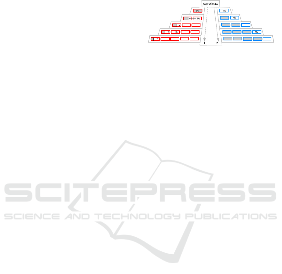
up, as shown in Fig. 1.
It evolves population at each level, until the pro-
motional criteria has been met and some part of the
population is promoted to the next level. The promo-
tional criterion is denoted by α and size of the pro-
moted population by β. Several variants of Pyramid
a
https://orcid.org/0000-0002-4661-1793
b
https://orcid.org/0000-0001-9818-911X
c
https://orcid.org/0000-0002-8182-2465
d
https://orcid.org/0000-0002-7002-5815
were examined, with levels varying from 2 to 5, re-
ferred to as HL-2 and HL-5 respectively. However, in
the case of 4 and 5 level Pyramid, the population size
(β) becomes very small at the final levels.
This paper attempts to automate the α and make
β less aggressive in reducing the population size for
the Pyramid, and to add a form of hyper-mutation at
the final level if there is still some budget left and the
fitness has not arrived at a satisfactory level (this takes
the form of increasing the mutation rate from 0.05 to
0.2). By satisfactory level, we mean that our approach
should outperform baseline.
The performance of proposed algorithm is mea-
sured using two unimodal and two multimodal func-
tions (the same as in (Ryan et al., 2020)) and we show
that our proposed new approach outperformed than
the traditional algorithm as well as the previous Pyra-
mid. We call our approach as Pyramid-Z.
In the next section, we highlight the existing hier-
archical techniques in EC and describe Pyramid and
its limitations. The proposed method is explained in
Section 3. We then present the experimental setup
in Section 4. Experimental results are discussed in
Section 5. Finally, Section 6 draws conclusions and
future work.
Rafiq, A., Naredo, E., Kshirsagar, M. and Ryan, C.
Pyramid-Z: Evolving Hierarchical Specialists in Genetic Algorithms.
DOI: 10.5220/0010657400003063
In Proceedings of the 13th International Joint Conference on Computational Intelligence (IJCCI 2021), pages 49-58
ISBN: 978-989-758-534-0; ISSN: 2184-3236
Copyright © 2023 by SCITEPRESS – Science and Technology Publications, Lda. Under CC license (CC BY-NC-ND 4.0)
49

2 BACKGROUND AND RELATED
WORK
2.1 Other Approaches
Based on the concept of Hierarchy, researchers have
experimented with different approaches to overcome
the scaling problems. These can be divided into three
broad categories:
Hierarchical Genetic Algorithms (HGAs). con-
sist of hierarchies of GAs that generally employ dif-
ferent fitness functions. Individuals can migrate up
(and occasionally down) through the various levels.
Several Studies (Sefrioui and P
´
eriaux, 2000), (Hong
et al., 2016), (Hong et al., 2017) (de Jong et al., 2004)
have employed hierarchy in GA and have achieved
promising results.
Incremental Evolution (IE). starts with a popula-
tion that is already trained on a simpler but related
task, rather than starting from initial random popu-
lation. Using this approach, many researchers (Bar-
low et al., 2004), (Winkeler and Manjunath, 1998),
(Duarte et al., 2012), (Assunc¸
˜
ao et al., 2020) have
been able to tackle difficult problems.
Layered Learning (LL). is an approach where
learning achieved at the lower layers helps facili-
tate learning required at upper layers. Various stud-
ies (Stone and Veloso, 1997),
(Astarabadi and Ebadzadeh, 2018),
(Jackson and Gibbons, 2007) have assessed the effi-
cacy of LL in order to overcome the bootstrapping
problems.
2.2 Pyramid
Pyramid (Ryan et al., 2020) is a Hierarchical Genetic
Algorithm that decomposes problems by first tackling
simpler versions of them, before automatically scal-
ing up to more difficult versions while also reduc-
ing the population size (shown in Fig. 1). It takes
inspiration from several systems, as it uses increas-
ingly more complex individuals as in (Astarabadi and
Ebadzadeh, 2018) and increasingly more precise fit-
ness functions as in (Sefrioui and P
´
eriaux, 2000).
Pyramid was constructed in such a way that the
smallest genome, largest population and simplest fit-
ness function are at the top, and the largest genome,
smallest population and most complex fitness func-
tion are at the bottom. With each step in the Pyramid,
the authors (Ryan et al., 2020) adjusted the population
Precise
Fitness
Function
H-L1
H-L2
H-L3
H-L4
H-L5
Genome Decomposition
Population Decomposition
g
3
g
5
p
2
p
4
Figure 1: Graphical representation of the Pyramid approach
with 5 levels. On the left side we see the population size
decreasing, while on the right, the genome length increases.
The fitness function gets increasingly more precise as we
descend (image taken from (Ryan et al., 2020)).
size down and the genome size up, because the longer
the individuals are, the more precise the fitness func-
tion is. Two important research questions in Pyramid
were (i) when should individuals be promoted to next
level; indicated by α and (ii) how many individuals
should be promoted; indicated by β.
The trigger point for promotion was that the top
20% of the population was five times better than the
average fitness of the population and these 20% were
the promoted individuals. In all but one problem,
Pyramid performed either the same or statistically sig-
nificantly better with substantially fewer evaluations.
2.3 Pyramid Drawbacks
In Pyramid, the choice of parameters (α and β) were
arbitrary. According to experimental results in the
original, in some problems, the population evolved
for hundreds of generations before meeting α but in
some problems, it took just a few generations.
Moreover, the choice of β led to a too-small pop-
ulation at the final levels. Although the evolution
started with 5000 individuals, the population size re-
duced to 40 and 8 in the final level of HL-4 (four level
Pyramid) and HL-5 (five level Pyramid) respectively.
This tiny population size sometimes does not contain
enough genetic material and population can easily be-
come stuck into local optima.
3 Pyramid-Z
Pyramid-Z addresses the limitations of Pyramid. The
right time about when to promote the individuals to
next level is determined using a new promotional cri-
teria α2 (explained in next Section 3.1). This param-
eter confirms that population has highly significantly
improved and now the individuals can be promoted to
next level to deal with another level of complexity.
In this parameter, the population in each gener-
ation is compared with the initial generation at that
ECTA 2021 - 13th International Conference on Evolutionary Computation Theory and Applications
50

level. If the population at that generation is signifi-
cantly better than the initial generation, then it is time
to promote individuals to next level.
Secondly, Pyramid-Z also ensures that there is a
sufficiently large population at final levels. This is
achieved using new parameter β2 (explained in Sec-
tion 3.2). Lastly, a new insight of increased mutation,
explained in Section 3.3, is incorporated for the cases
where Pyramid-Z has not attained a satisfactory fit-
ness. Note that (α 2, β2) replace (α, β); we use differ-
ent names in this paper to facilitate comparison. Fig. 2
depicts the logic of the Pyramid-Z.
3.1 α2
We replace the arbitrary α parameter with a statistical
test that tests if two distributions are equal or different
from one another, specifically, the Z-test:
Z =
(
¯
X
1
−
¯
X
2
)
r
(
σ
X
1
√
n
1
)
2
+ (
σ
X
2
√
n
2
)
2
(1)
where X
1
is the initial distribution (initial generation,
at each level, in our case) and
¯
X
1
is its mean value.
X
2
is the second distribution (each next generation in
our case) and
¯
X
2
is its mean value. σ
X
1
is the standard
deviation of distribution X
1
and then it is divided by
the square root of the number of data points (n is the
population size of each distribution in our case).
σ
X
2
is the standard deviation of distribution X
2
and
then it is divided by the square root of the number of
data points. Based on the value of Z-test, as shown in
Table 1, one can see how much the distributions differ
from each other. The Z-test is applied at each gener-
ation against the initial generation at that level. If the
value of Z at a certain generation is greater than 3,
then it means that the two generations are highly sig-
nificantly different from each other. Here, by different
we assume the improvements. Now, at that specific
generation, we stop the current level and promote the
individuals to next level.
Table 1: Meaning of Z-test. In our experiments, we choose
the >3 to make sure that two populations are highly signif-
icantly different from each other.
Z-test Value Statistical Interpretation
<2.0 Same
2.0 - 2.5 Marginally Different
2.5 - 3.0 Significantly Different
>3.0 Highly Significantly Different
3.2 β2
Recall that the issue with β was that it could be too ag-
gressive in reducing the population size. We replace
this with a more gradual decrease in which we spec-
ify the total number of levels (L), the initial popula-
tion size (P
initial
) and the final population size (P
f inal
).
Then, we propose a way of reducing the population
(D) at each level by using the algorithm 1.
Algorithm 1: How population size varies at each level.
1 D =
j
P
initial
−P
f inal
L−1
k
2 i = 1;
3 while i¡L do
4 P
new
= P
c
−D;
5 P
c
= P
new
;
6 i + +;
7 end
Where P
new
is the new population at the next level.
3.3 Hyper-mutation
After applying the parameters (α and β) and get-
ting the initial results, we identify the cases where
Pyramid-Z has not reached its desired goal. By de-
sired goal, we mean that our approach should outper-
form baseline. In these cases, we increase the mu-
tation rate from 0.05 to 0.2 for the population at the
final level and let the population evolve again. This
increased mutation ratio is chosen to fit with our other
parameters (crossover rate, population size etc.) in ac-
cordance with (Hassanat et al., 2019) where authors
have reviewed several methods for choosing the mu-
tation and crossover rations in GAs. From Fig. 2, the
highlighted area in red color is where the population
gets another chance to evolve, when under-performed
than baseline.
4 EXPERIMENTAL SETUP
As discussed in Section 2.2, two important research
questions in Pyramid are indicated by (α, β) (shown
in Table 2). Here, (α1, β1) were the original ap-
proaches, used in (Ryan et al., 2020), while (α2, β2)
are those explored in this paper. By using the combi-
nation of both (α, β), four experiments were run such
as (α1, β1) (Experiment 1), (α2, β1) (Experiment 2),
(α1, β2) (Experiment 3) and (α2, β2) (Experiment 4).
Pyramid-Z: Evolving Hierarchical Specialists in Genetic Algorithms
51

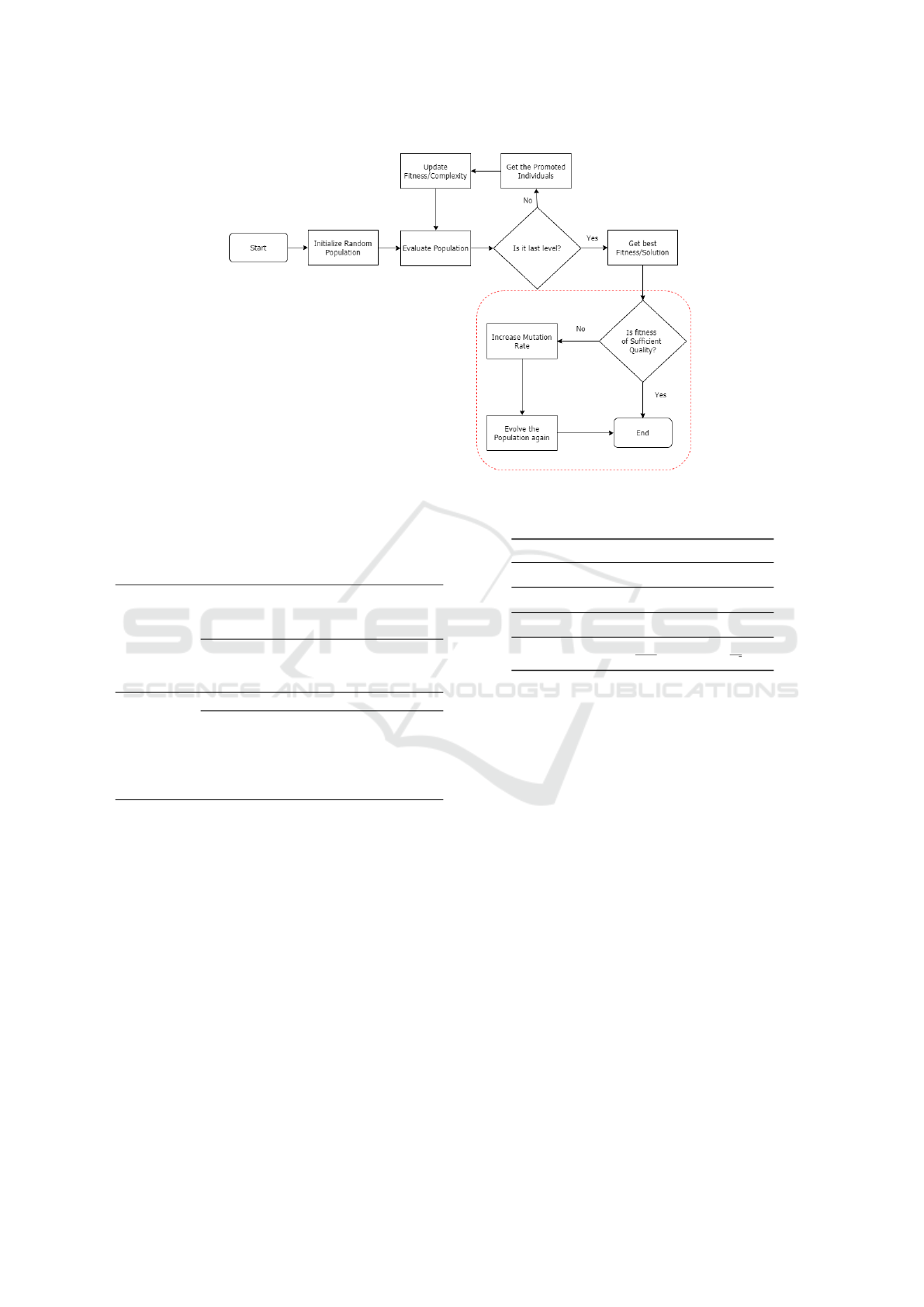
Figure 2: Pyramid-Z Flow Chart, the highlighted red dot area is where Pyramid-Z enters a period of hyper-mutation.
Table 2: A comparison of the approaches. The upper
two rows show the alternative ways to promote individu-
als while, the number of individuals to promote are in the
lower two. In the previous Pyramid, (α1, β1) were used.
Promotional
Criteria
(α)
α1
Top 20% of the population is five
times better than the average
fitness of the population.
α2
When the value of z is greater
than 3, explained
in Section 3.1.
Population
Threshold
(β)
β1 20% of the top population.
β2
Size of promoted individuals varies
according to number of
levels and initial/final
population size,
explained in Section 3.2.
4.1 Problems
Four mathematical functions, two uni-modal (Sphere
and Rosenbrock) and two multi-modal (Rastrigin and
Griewank), as shown in Table 3, were chosen to test
the performance of our algorithm. These functions are
well-known optimization problems (Jamil and Yang,
2013) and have been frequently used in other hierar-
chical studies (Hong et al., 2016) (Hong et al., 2017).
The optimal value for all these functions is 0.
The experimental setup is graphically summarized
in the Fig. 3 showing the four versions tested for
Pyramid-Z applied on four problems (two unimodal
and two multimodal) and each problem is tested with
four variants of Pyramid-Z (from HL-2 to HL-5). All
those cases, where Pyramid-Z out-performed than the
baseline is highlighted in green and those cases are
Table 3: Benchmark Functions.
Name Function
Sphere
∑
n
i=1
x
2
i
Rosenbrock
∑
n−1
i=1
[100(x
i+1
−x
2
i
)
2
+ (x
i
−1)
2
]
Rastrigin 10n +
∑
n
i=1
(x
2
i
−10cos(2πx
i
))
Griewank 1 +
∑
n
i=1
x
2
i
4000
−
∏
n
i=1
cos(
x
i
√
i
)
shown in the section of the experimental results.
We used OpenGA (Mohammadi et al., 2017), an
open source C++ library for GAs to implement this
version of Pyramid.
5 EXPERIMENTAL RESULTS
AND ANALYSIS
5.1 Experiments
Initially, a baseline experiment was run using a tra-
ditional GA, followed by four variants of our ex-
periment and each experiments has four variants of
our Pyramid-Z, each with varying levels (2 to 5), as
shown in Table 4. These are referred to as H-LX
where X is the number of levels in the hierarchy.
5.2 Results
The correlation between the best fitness and the num-
ber of individuals processed were tested. All these
results are the average of 50 runs. We describe the
results for each problem separately below.
ECTA 2021 - 13th International Conference on Evolutionary Computation Theory and Applications
52

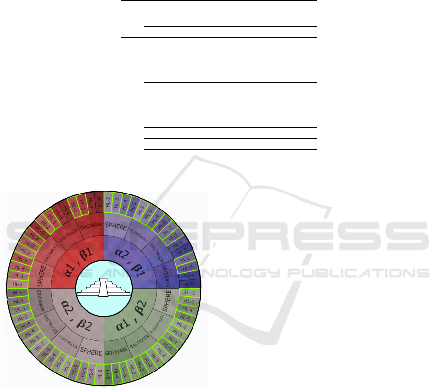
Table 4: Parameters for Pyramid-Z: The target genome length for each H-LX is 30, which is divided into different values
according to specific experiment. The values for Chromosome length that show a calculation refer to the previous length plus
the additional length, e.g. 20+10=30 means the previous length was 20 and we are adding 10 more to give a length of 30. β1
and β2 are the ways in which the population size varies at each level. β1 promotes 20% population size to next level, while
β2 assures that the minumum population size at the final level is 200.
Level Chrom. length β1 β2 Max-Gener
Baseline 30 5,000 5,000 3,000
H-L2
L1 15 5,000 5,000 1,500
L2 15+15=30 1,000 200 1,500
H-L3
L1 10 5,000 5,000 1,000
L2 10+10=20 1,000 2600 1,000
L3 20+10=30 200 200 1,000
H-L4
L1 7 5,000 5,000 700
L2 7+8=15 1,000 3400 800
L3 15+7=22 200 1800 700
L4 22+8=30 40 200 800
H-L5
L1 6 5,000 5,000 600
L2 6+6=12 1,000 3800 600
L3 12+6=18 200 2600 600
L4 18+6=24 40 1400 600
L5 24+6=30 8 200 600
Figure 3: Mayan-like calendar showing all experiments
with Pyramid-Z. Each quadrant with different color shows
a combination of (α, β) parameters. There are four sections
in the quadrants corresponding to the optimization prob-
lem addressed and each sub-section shows the four levels
of complexity decomposition for each of them. All levels
where Pyramid-Z outperform the baseline are outlined in
green.
5.2.1 Sphere
Table 5 shows the statistical comparison. The ta-
ble divides the results into two groups. In the first
group, we have Individuals Processed and the average
and standard deviation of the fitness. In the second
group, hyper-mutation kicked in, in all those cases
where Pyramid-Z required extra evaluations. In base-
line, the number of individuals processed is shown in
bold 651,749. This is actually the budget limit for this
problem. As can be seen from the table that HL-4 and
HL-5 Pyramid-Z under-performed than the baseline
in (α1, β1) and (α2, β1) setup respectively. In those
cases, we show updated values of fitness and standard
deviation after hyper-mutation kicked in. Although
the budget has increases (more individuals have been
processed), these cases now out-perform the baseline.
All the bold values in the table shows where the var-
ious Pyramids out-performed than the baseline. For
the statistical analysis, t-test was used, which returns
the p-value < 0.01 in all the cases.
Fig. 4 compares the values of fitness and individu-
als processed. The resulting values from Table 5 are
normalized from 0 to 1 in order to visualize better.
The figure has two parts, part (a) compares the fitness
values of each of our experiment with Baseline and
the part (b) compares the number of individuals pro-
cessed. From part (b) of each figure, we can clearly
see that the number of individuals processed in our
experiments are much smaller than the baseline and
from part (a) it is also clear that the fitness in all our
experiments is better than the baseline. All our cases,
out-performed in Sphere function.
Pyramid-Z: Evolving Hierarchical Specialists in Genetic Algorithms
53

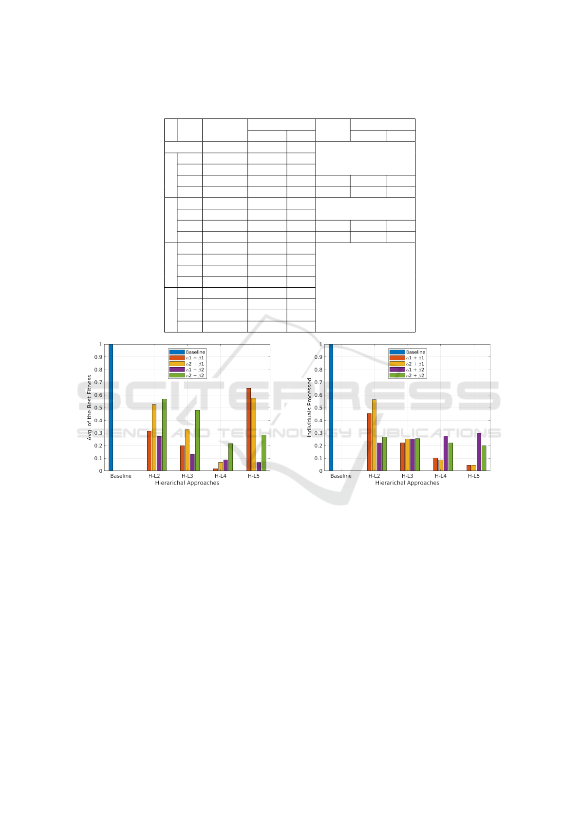
Table 5: Results from the Sphere function. + indicates Pyramid-Z performed statistically significantly better, - that Pyramid-Z
performed statistically significantly worse. In all - cases, the budget has been increased and results improve.
H-LX
Individuals
Processed
Best Fitness Updated
Budget
Updated Fitness
Avg std Avg std
Baseline 651,749 1.0012 0.0784
α1
β1
H-L2 37,049 0.5644 + 0.0523
H-L3 36,680 0.3547 + 0.0867
H-L4 34,892 5.8534 - 2.7289 60,252 0.0292 + 0.0310
H-L5 30,375 15.9313 - 5.6826 62,583 1.1700 + 0.6292
α2
β1
H-L2 410,000 0.9403 + 0.1805
H-L3 185,200 0.5847 + 0.1832
H-L4 43,680 2.7202 - 1.5829 84,840 0.1241 + 0.2899
H-L5 20,392 4.5929 - 4.5929 52,792 1.0315 + 0.5181
α1
β2
H-L2 194,600 1.0213 + 0.3534
H-L3 186,600 0.8599 + 0.2860
H-L4 161,400 0.3873 + 0.0743
H-L5 144,600 0.5058 + 0.1408
α2
β2
H-L2 162,200 0.4896 + 0.1306
H-L3 184,800 0.2327 + 0.0423
H-L4 20,800 0.1601 + 0.0315
H-L5 218,400 0.1195 + 0.0215
(a) Fitness (b) Individuals Processed
Figure 4: Sphere Results: The fitness value and number of individuals processed of baseline is compared against our experi-
ments, on left and right hand side respectively. It can be clearly seen that that fitness value in our experiment is always better
than baseline (a) and always with less individuals processed (b).
5.2.2 Rosenbrock
Table 6 shows the various results. In the first group,
we can see the Pyramid-Z did not perform well in
most cases. With hyper-mutation, all the cases now
out-performed except HL-5 in both (α1, β1) and (α2,
β1) setup. This is due to the way β1 behaves as it
reduces the population size to very small (can also be
seen from Table 4) at the final level of HL-5. All cases
where Pyramid-Z out-performed are shown in bold.
Similarly, Fig. 5 compares the fitness and number of
individuals processed from part (a) and part (b) re-
spectively. In rosenbrock, all the cases out-performed
except HL-5 in both (α1, β1) and (α2, β1).
5.2.3 Rastrigin
Table 7 shows the results. We can see that in first
part of the table Pyramid-Z did not perform as well as
the baseline, albeit with far fewer evaluations. This
is where again the hyper-mutation plays its part. We
increased the budget and can see that our Pyramids
now start out-performing. Fig. 6 compares the fit-
ness and number of individuals processed from part
(a) and part (b) respectively. Rastrigin function out-
performed in all the cases except HL-4 and HL-5 in
both (α1, β1) and (α2, β1) setup.
ECTA 2021 - 13th International Conference on Evolutionary Computation Theory and Applications
54

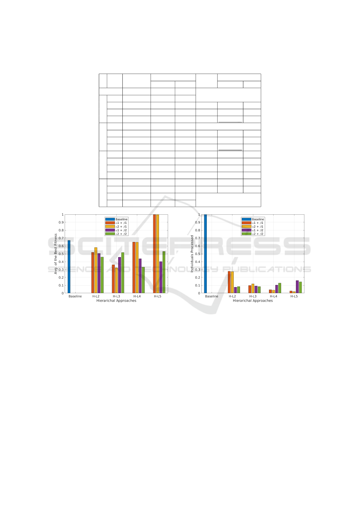
Table 6: Results from the Rosenbrock function. + indicates Pyramid-Z performed statistically significantly better, - that
Pyramid-Z performed statistically significantly worse. In all - cases, the budget has been increased and results improve.
H-LX
Individuals
Processed
Best Fitness Updated
Budget
Updated Fitness
Avg std Avg std
Baseline 920,000 70.658 5.622
α1
β1
H-L2 254,000 54.522 + 4.248
H-L3 71,800 84.457 - 14.639 109,600 37.807 + 7.869
H-L4 21,560 248.277 - 68.201 59,280 68.2384 + 25.593
H-L5 19,320 394.118 - 167.147 45,040 104.822 - 28.200
α2
β1
H-L2 252,000 60.950 + 6.347
H-L3 66,000 100.524 - 22.146 119,000 33.894 + 5.112
H-L4 16,640 253.094 - 50.998 47,640 68.006 + 23.231
H-L5 13,184 381.126 - 125.725 31,920 105.071 - 46.524
α1
β2
H-L2 69,000 102.970 - 20.940 88,400 53.129 + 16.017
H-L3 63,000 98.484 - 20.763 105,200 48.022 + 14.021
H-L4 72,400 92.833 - 21.109 137,600 46.025 + 9.537
H-L5 80,600 111.512 - 33.328 204,800 42.342 + 9.739
α2
β2
H-L2 71,200 97.347 - 22.984 85,600 48.302 + 12.590
H-L3 85,800 74.855 - 14.187 105,400 54.2198 + 19.872
H-L4 93,600 67.200 + 12.111
H-L5 109,600 61.633 + 9.371
(a) Fitness (b) Individuals Processed
Figure 5: Rosenbrock Results: The fitness value and number of individuals processed of baseline is compared against our
experiments, on left and right hand side respectively. It can be clearly seen that that fitness value for Pyramid-Z is always
better, except in two cases (a), and our experiments always processed less individuals (b).
5.2.4 Griewank
Table 8 is the comparison of statistical values. We
can see that our experiment did not perform well in
all cases. Now, when we increased the budget and
let the population evolve again, we can see the almost
all cases are out-performing. These results are similar
to Rastrigin, as Pyramid-Z out-performed in all cases
except HL-4 and HL-5 in both (α1, β1) and (α2, β1)
setup.
Overall, these results show that Pyramid-Z out-
performed in most cases. One possible reason where
Pyramid-Z did not perform well is the choice of β1.
According to this parameter, the population size is
very small in the last level (40 and 8 for HL-4 and HL-
5 respectively), so there is not enough genetic mate-
rial. Interestingly, most of the cases now outperforms
baseline.
In summary, all the results are shown in the form of
a hierarchical pie chart from Fig. 3. The hierarchi-
cal pie chart briefly summarizes the experimentation
results for the system Pyramid-Z. Two Unimodal and
two multimodal sample problems were tested for each
of the four budget scenarios for (α, β). For example,
for the case with (α1, β1) the Pyramid-Z achieved op-
timal solution at all 2-5 levels Pyramids for sphere, for
Rosenbrock at 2-4 levels Pyramid, for both Rastrigin
and Griewank at 2 and 3 levels. The best performing
Pyramid-Z: Evolving Hierarchical Specialists in Genetic Algorithms
55

Table 7: Results from the Rastrigin function. + indicates Pyramid-Z performed statistically significantly better, - that
Pyramid-Z performed statistically significantly worse. In all - cases, the budget has been increased and results are better.
H-LX
Individuals
Processed
Best Fitness Updated
Budget
Updated Fitness
Avg std Avg std
Baseline 2,110,000 15.0649 3.0383
α1
β1
H-L2 886,000 11.3094 + 5.6589
H-L3 590,400 16.0864 - 9.0095 1,053,600 10.5174 + 4.7767
H-L4 383,720 41.3362 - 13.8260 791,520 20.8209 - 6.9686
H-L5 279,968 57.4871 - 15.2764 576,304 30.9646 - 12.1054
α2
β1
H-L2 1,085,000 20.4950 - 5.0858 1,134,000 13.6199 + 13.9235
H-L3 205,800 47.9625 - 12.2669 283,000 11.5174 + 5.7167
H-L4 18,560 204.9727 - 35.6858 74,040 60.6924 - 31.8871
H-L5 13,312 234.1956 - 26.4372 51,520 68.4385 - 23.6885
α1
β2
H-L2 253,200 48.4930 - 29.6217 506,200 14.9440 + 5.7609
H-L3 195,200 47.7511 - 23.1457 674,600 8.2364 + 3.7970
H-L4 164,200 58.3643 - 30.8686 686,200 5.8924 + 3.3659
H-L5 120,800 90.2085 - 45.4135 597,400 4.6677 + 2.2798
α2
β2
H-L2 458,400 21.3997 - 9.4226 488,400 9.2264 + 3.7090
H-L3 584,400 12.5549 + 6.3339
H-L4 622,600 9.5348 + 5.6753
H-L5 530,600 8.4187 + 4.5301
(a) Fitness (b) Individuals Processed
Figure 6: Rastrigin Results: The fitness value and number of individuals processed of baseline is compared against our
experiments, on left and right hand side respectively. It is clearly seen that fitness value in our experiment is always better,
except in 4 cases, than baseline (a) but our experiments always processed less individuals (b).
levels for each set of problems are highlighted.
Similarly, we can observe that for scenario (α2,
β2) and (α1, β2) the Pyramid-Z started outperform-
ing the baseline from 2 level itself and consistently
maintained the trend of reaching optimal solutions at
subsequent higher levels. Finally, Table 9 summa-
rizes about a comparison between the Traditional ap-
proach, Pyramid and Pyramid-Z.
6 CONCLUSIONS AND FUTURE
WORK
In this paper, we present the new version of previ-
ously proposed Pyramid, called Pyramid-Z. Two key
parameters of Pyramid, i.e. when to promote and
how many individuals to promote, are tackled here.
The first parameter from the original version was re-
placed by Z-test to identify when the current popu-
lation is highly significant different from the origi-
nal one on each hierarchical level and thus automate
the promotional time, and second one made less ag-
ECTA 2021 - 13th International Conference on Evolutionary Computation Theory and Applications
56

Table 8: Results from the Griewank function. + indicates Pyramid-Z performed statistically significantly better, - that
Pyramid-Z performed statistically significantly worse. In all - cases, the budget has been increased and results improve.
H-LX
Individuals
Processed
Best Fitness Updated
Budget
Updated Fitness
Avg std Avg std
Baseline 6,517,491 1.0533 0.0802
α1
β1
H-L2 1,369,560 1.8770 - 0.5976 1,943,560 0.0287 + 0.2520
H-L3 176,310 6.3616 - 1.9758 693,110 1.0931 + 0.4826
H-L4 30,946 23.0932 - 0.0784 478,826 5.0645 - 2.2795
H-L5 91,126 37.9472 - 12.6262 439,638 9.4037 - 5.5654
α2
β1
H-L2 1,433,000 2.0789 - 0.6747 2,025,000 0.2976 + 0.2193
H-L3 187,400 7.8081 - 2.1759 749,400 1.0755 + 0.0927
H-L4 24,880 31.3044 - 8.8449 524,560 7.2382 - 3.1412
H-L5 19,376 50.0469 - 15.2384 392,080 11.6984 - 6.8497
α1
β2
H-L2 235,400 11.3947 - 3.2584 842,400 1.0880+ 0.4682
H-L3 187,000 9.7794 - 2.6214 704,400 1.4201 + 0.5574
H-L4 159,400 9.5497 - 3.0016 593,200 0.6665 + 0.2807
H-L5 130,200 17.6775 - 4.9375 183,900 1.0750 + 0.3659
α2
β2
H-L2 234,800 10.6573 - 3.7879 918,600 0.3916 + 0.2993
H-L3 202,800 5.7381 - 1.8355 823,600 0.7615 + 0.3601
H-L4 215,800 3.2703 - 1.1426 835,400 0.2171 + 0.2913
H-L5 205,600 4.2385 - 1.3597 1012,600 1.0701 + 0.4574
(a) Fitness (b) Individuals Processed
Figure 7: Griewank Results: The fitness value and number of individuals processed of baseline is compared against our
experiments, on left and right hand side respectively. It is clearly seen that that fitness value in our experiment is always
better, except 4 cases, than baseline (a) but our experiments always processed less individuals (b).
Table 9: Comparative Analysis of Traditional Approach
with Pyramid and Pyramid-Z.
Methods Results/Findings
Traditional GA
Processes a large number of individuals
to obtain optimal solutions.
Pyramid
Approximately 98% reduction in individuals
being processed but does not guarantee
optimal solutions always.
Pyramid-Z
90% reduction in individuals processed
and also guarantees to always obtain
optimal solution
gressive to maintain a moderate population size. The
proposed new changes make the Pyramid-Z more ef-
ficient based on the results. As previous Pyramid,
we always processed fewer individuals than the tra-
ditional algorithm processed.
We exploit the fact that we have so few individu-
als processed in the case where Pyramid-Z gets stuck
to enter a new phase of evolution driven by hyper-
mutation. Our results show that this almost always
improves performance relative to standard approaches
while still using significantly fewer evaluations.
Currently Pyramid-Z is only defined for real
coded GAs. Future work will explore programming
problems where the complexity of the problem will
need to be moderated solely by the fitness function.
Pyramid-Z: Evolving Hierarchical Specialists in Genetic Algorithms
57

REFERENCES
Assunc¸
˜
ao, F., Lourenc¸o, N., Ribeiro, B., and Machado, P.
(2020). Incremental evolution and development of
deep artificial neural networks. In European Con-
ference on Genetic Programming (Part of EvoStar),
pages 35–51. Springer.
Astarabadi, S. S. M. and Ebadzadeh, M. M. (2018). A
decomposition method for symbolic regression prob-
lems. Applied Soft Computing, 62:514–523.
Barlow, G. J., Oh, C. K., and Grant, E. (2004). Incre-
mental evolution of autonomous controllers for un-
manned aerial vehicles using multi-objective genetic
programming. In Cybernetics and Intelligent Systems,
2004 IEEE Conference on, volume 2, pages 689–694.
IEEE.
de Jong, E. D., Thierens, D., and Watson, R. A. (2004). Hi-
erarchical genetic algorithms. In International Con-
ference on Parallel Problem Solving from Nature,
pages 232–241. Springer.
Duarte, M., Oliveira, S., and Christensen, A. L. (2012).
Hierarchical evolution of robotic controllers for com-
plex tasks. In 2012 IEEE International Conference on
Development and Learning and Epigenetic Robotics
(ICDL), pages 1–6. IEEE.
Hassanat, A., Almohammadi, K., Alkafaween, E.,
Abunawas, E., Hammouri, A., and Prasath, V. (2019).
Choosing mutation and crossover ratios for genetic al-
gorithms—a review with a new dynamic approach. In-
formation, 10(12):390.
Hong, T.-P., Peng, Y.-C., and Lin, W.-Y. (2016). Multi-
population genetic algorithm with hierarchical execu-
tion. In 2016 International Conference on Fuzzy The-
ory and Its Applications (iFuzzy), pages 1–4. IEEE.
Hong, T.-P., Peng, Y.-C., Lin, W.-Y., and Wang, S.-L.
(2017). Empirical comparison of level-wise hierar-
chical multi-population genetic algorithm. Journal of
Information and Telecommunication, 1(1):66–78.
Jackson, D. and Gibbons, A. P. (2007). Layered learning
in boolean gp problems. In European Conference on
Genetic Programming, pages 148–159. Springer.
Jamil, M. and Yang, X.-S. (2013). A literature survey
of benchmark functions for global optimization prob-
lems. arXiv preprint arXiv:1308.4008.
Mohammadi, A., Asadi, H., Mohamed, S., Nelson, K., and
Nahavandi, S. (2017). openga, a c++ genetic algo-
rithm library. In 2017 IEEE International Confer-
ence on Systems, Man, and Cybernetics (SMC), pages
2051–2056. IEEE.
Ryan, C., Rafiq, A., and Naredo, E. (2020). Pyramid: A hi-
erarchical approach to scaling down population size in
genetic algorithms. In 2020 IEEE Congress on Evolu-
tionary Computation (CEC), pages 1–8. IEEE.
Sefrioui, M. and P
´
eriaux, J. (2000). A hierarchical genetic
algorithm using multiple models for optimization. In
International Conference on Parallel Problem Solving
from Nature, pages 879–888. Springer.
Stone, P. and Veloso, M. (1997). A layered approach to
learning client behaviors in the robocup soccer server.
Computer Science, 412:268–7123.
Winkeler, J. F. and Manjunath, B. (1998). Incremental
evolution in genetic programming. Genetic Program-
ming, pages 403–411.
ECTA 2021 - 13th International Conference on Evolutionary Computation Theory and Applications
58