Multivariate Short Term Load Forecasting Strategy: Application to
Anomalous Days of ISO New England Data
Innocent Sizo Duma
1
and Bhekisipho Twala
2
1
Department of Electrical Power Engineering, Faculty of Engineering and the Built Environment,
Durban University of Technology, P.O. Box 1334, Durban, 4000, South Africa
2
Faculty of Engineering and the Built Environment, Durban University of Technology,
P.O. Box 1334, Durban, 4000, South Africa
Keywords:
Short Term Load Forecasting, Multivariate Denoising using Wavelet and Principal Component Analysis,
Bayesian Optimization Algorithm, Long Short-Term Memory Neural Networks, Feedforward Neural
Networks, Random Forest.
Abstract:
In this paper, we consider short-term electricity load forecasting which is for making forecasting within 1 hour
to 7 days or a month ahead usually used for the day-to-day operations of the utility industry, such as schedul-
ing the generation and transmission of electric energy. This is a three step process: (1) Data preprocessing
which include feature extraction, (2) Modeling and (3) Model Evaluation. Electrical load time series are non
stationary and notoriously very noisy because of variety of factors that affect the electrical markets. As a data
preprocessing step to remove the white noise on the multivariate predictor variables (which include historical
load, weather, and holidays) we perform a multivariate denoising using wavelets and principal component
analysis (MWPCA). In the modeling step we propose three multivariate Bayesian Optimization (BO) based
Random Forest (RF), Feedforward Neural Networks (FFNN) and Long Short-term Memory (LSTM) neural
network for day ahead hourly load forecast of the anomalous days system load of the ISO New England grid.
For model evaluation we used three evaluation metrics, the Mean Absolute Percent Error (MAPE), Mean Ab-
solute Error (MAE), and Root Mean Square Error (RMSE). All the trained models achieved a superior results
on the chosen model evaluation metrics most notably achieving a MAPE of less than 1% on the data under
study. And the FFNN model outperformed both the RF and LSTM models.
1 INTRODUCTION
Load forecasting is a central and integral process in
the planning and operation of electric utilities. It in-
volves the accurate prediction of both the magnitudes
and geographical locations of electric load over the
different periods (usually hours) of the planning hori-
zon. The basic quantity of interest in load forecast-
ing is typically the hourly total system load. How-
ever , load forecasting is also concerned with the pre-
diction of hourly, daily, weekly and monthly values
of the system load, peak system load and the system
energy. Load forecasting can be classified in terms
of the planning horizon’s duration: up to 1 hour for
very short-term load forecasting (VSTLF), 24 hours
to one week for short-term load forecasting (STLF),
more than one week to few months for medium-term
load forecasting (MTLF), and 1±10 years for long-
term load forecasting (LTLF).
Accurate load forecasting holds a great saving po-
tential for electric utility corporations, these savings
are realised when load forecasting is used to control
operations and decisions such as dispatch, unit com-
mitment, fuel allocation and off-line network analy-
sis. The accuracy of load forecasts has a significant
effect on power system operations, as economy of op-
erations and control of power systems may be quite
sensitive to forecasting errors. It is observed that both
positive and negative forecasting errors resulted in in-
creased operating costs. Hobbs (Hobbs et al., 1999)
quantified the dollar value of improved Short Term
Load Forecasting for a typical utility and observed
that a 1% reduction in the average forecast error for
a 10, 000MW utility can save up to $1.6 million an-
nually and that was 22 years ago.
Previous work has been carried out on Short term
load forecasting for Anomalous Days of ISO New
England Grid Data by Raza (Raza et al., 2020) who
proposed an ensemble forecast framework with a sys-
Duma, I. and Twala, B.
Multivariate Short Term Load Forecasting Strategy: Application to Anomalous Days of ISO New England Data.
DOI: 10.5220/0010652600003063
In Proceedings of the 13th International Joint Conference on Computational Intelligence (IJCCI 2021), pages 293-301
ISBN: 978-989-758-534-0; ISSN: 2184-3236
Copyright © 2023 by SCITEPRESS – Science and Technology Publications, Lda. Under CC license (CC BY-NC-ND 4.0)
293

tematic combination of three predictors, namely El-
man Neural Network (ELM), Feedforward Neural
Network (FFNN) and Radial Basis Function (RBF)
Neural Network. They trained these predictor models
using Global Particle Swarm Optimization (GPSO)
to improve their training capability in the ensemble
framework. The outputs of individual predictors were
combined using trim aggregation technique by re-
moving forecating anomalies. Their predictor vari-
ables which include weather, seasonality and histori-
cal load were subjected to univariate wavelet denois-
ing to remove fluctuations and spikes. Their proposed
model showed a significant improvement in predic-
tion accuracy compared to autoregressive integrated
moving average (ARIMA) and back-propagationneu-
ral networks (BPNN).
As Raza (Raza et al., 2020) put it succinctly: “
For load forecasting of a normal day, a day with a
predictable load profile, the training data have enough
correlated training samples to train the model. How-
ever, an anomalous day load forecasting has a much
smaller number of patterns for effective training of
the model. Therefore, the anomalous day forecast-
ing model is more complex and difficult to design
for higher forecast accuracy. Generally, the predic-
tion accuracy of models for anomalous days is lower
due to multiple factors such as uncertainty in de-
mand, meteorological variables, unpredictable socio-
logical events and intermittency of renewable energy
resources etc.” It is these challenges that encourages
us to put foward our methodology.
Nti (Nti et al., 2020) undertook a systematic and
critical review of about seventy-seven (77) relevant
previous works reported in academic journals over
nine years 2010 − 2020 in electricity load forecast-
ing. Specifically, attention was given to the follow-
ing themes: (i) The forecasting algorithm used and
their fitting ability in this field, (ii) the theories and
factors affecting electricity consumption and the ori-
gin of research work, (iii) the relevant accuracy and
error metrics applied in electricity load forecasting,
and (iv) the forecasting period. Their results revealed
that 90% out of the top nine models used in electric-
ity load forecasting where artificial intelligence based,
with Artificial Neural Networks (ANN) representing
28%. They also observed that ANN models were pri-
marily used for short-term electricity load forecasting
where electrical energy consumptionare complicated.
Son (Son and Kim, 2020) proposed a LSTM
model that can accurately forecast monthly residen-
tial electricity demand and compared its performance
to four benchmark models: Support Vector Regres-
sion, Artificial Neural Network (ANN), Autoregres-
sive Integrated Moving Average (ARIMA) and Mul-
tiple Linear Regression. The LSTM model showed
a superior performance for MAPE by achieving the
lowest MAPE value, of less or equal to 1%.
A comparative analysis of five commonly used
short-term load forecasting techniques, i.e. Auto-
Regressive Integrated Moving Average (ARIMA),
Multiple Linear Regression (MLR), Recursive Parti-
tioning Regression Trees with Bootstrap Aggregating
(RPART+BAGGING), Conditional Inference Trees
with Bootstrap Aggregating (CTREE+BAGGING),
and Random Forest (RF) was performed by Kapoor
(Kapoor and Sharma, 2018). On comparison of
MAPE of all techniques, they concluded that the error
associated with RF was least and this approach pro-
duced more accurate results. A comparative study by
Kandananond (Kandananond, 2011), in which three
methodologies, ARIMA, ANN and Multiple Linear
Regression (MLR) were deployed to load forecast-
ing in Thailand. The results showed that the ANN
model reduced the MAPE to 0.996%, while those of
ARIMA and MLR were 2.80981% and 3.2604527%
respectively.
Rana (Rana and Koprinska, 2016) presented an
approach for very short-term load forecasting called
Advanced Wavelet Neural Networks (AWNN) which
used a shift invariant advanced wavelet packet trans-
form for load decomposition, Mutual Information for
feature selection and a multi-layer perceptron Neu-
ral Network trained with Levenberg-Marquardt algo-
rithm for prediction. They evaluated the performance
of their AWNN model using two different datasets for
two years: Australian 5-min data and Spanish 60-min
data. They choose the different geographic location
and time resolution to better access the robustness of
their AWNN model. Using the two evaluation met-
rics MAE and MAPE their AWNN models outper-
formed a number of methods used for comparison:
three ARIMA methods, three Holt-Winters exponen-
tial smoothing methods, an industry model, several
na¨ıve baselines, and also single non-wavelet Neural
Networks, Linear Regression, and Model Tree Rule.
Wang (Wang et al., 2014) proposed a novel ap-
proach for short-term load forecasting by applying
univariate wavelet denoising in a combined model
that is a hybrid of the seasonal autorgressive in-
tegrated moving average (SARIMA) model and a
back propagation neural networks (BPNN). Electric-
ity load data from New South Wales, Australia was
used to evaluate the performance of their proposed
approach. They compare their combined model with
the SARIMA, and BPNN and the results showed
that their proposed model can effectively improve the
forecasting accuracy.
NCTA 2021 - 13th International Conference on Neural Computation Theory and Applications
294

Munem (Munem et al., 2020) proposed a multi-
variate Bayesian Optimization based Long short-term
memory (LSTM) neural network to forecast the res-
idential electric power load for the upcoming hour.
Their model surpasses convolutional neural network
(CNN), artificial neural network (ANN) and support
vector machine (SVM) using MAE, RMSE and MSE
(Mean Squared Error) as performance evaluation met-
rics. They also observed that though their model per-
formed conspicuously it can be improved by adding
feature selection technique with the model.
Overview. The main objective of this study is to
achieve a MAPE of less than 1% on day ahead hourly
load forecast of the Anomalous Days of ISO New
England Grid Data. To this period no monogram in
short term load forecasting has combined Multivari-
ate Denoising Using Wavelet and Principal Compo-
nent Analysis with Bayesian Optimization for model
hypeparameter tuning and this work seeks to fill in
that gap.
Section 2 briefly discusses Multivariate Denois-
ing Using Wavelet and Principal Component Analy-
sis, Bayesian Optimization for Hyperparameter Tun-
ing, the three models used in this study Random For-
est (RF), Feedforward Neural Networks (FFNN), and
the Long Short Term Memory (LSTM) Neural Net-
work.
Section 3 outlines the methodology followed in
this study.
Section 4 outlines the experiments and findings
of this study with regards to the objective specified
above.
Section 5 concludes the paper and outlines future
directions.
2 BACKGROUND
In this section, we briefly describe Multivariate De-
noising Using Wavelet and Principal Component
Analysis, Bayesian Optimization for model hypepa-
rameter tuning, Random Forest, Feedforward Neu-
ral Network (FFNN) and Long Short-Term Memory
(LSTM) Neural Network.
2.1 Multivariate Wavelet Denoising
using Principal Component Analysis
The Multivariate Denoising Using Wavelet and Prin-
cipal Component Analysis Scheme of Aminghafari
(Aminghafari et al., 2006) is performed by the MAT-
LAB R2020b function WMULDEN and outlined in
Algorithm 1: Multivariate Denoising Using Wavelet and
Principal Component Analysis (WPCA).
• Parameters: J ∈ N.
1: Apply the level J wavelet decomposition of each
column of X, where X is an n× p predictor ma-
trix. This step produces J + 1 matrices D
1
, . . . , D
J
containing the detail coefficients at level 1 to J of
the p signals and the approximation coefficients
A
J
of the p signals. Matrices D
j
, 1 ≤ j ≤ J, and
A
J
are, respectively, of size
n
2
j
× p and
n
2
J
× p.
2: State
ˆ
Σ
ε
the estimator of Σ
ε
, the noise covari-
ance matrix, equivalent to the Minimum Co-
variance Determinant estimator (MCD) as
ˆ
Σ
ε
=
MCD(D
1
) and then compute the Singular Value
Decomposition (SVD) of
ˆ
Σ
ε
providing an or-
thogonal matrix V such that
ˆ
Σ
ε
= VΛV
T
where
Λ = diagonal(λ
i
, 1 ≤ i ≤ p). Apply to each detail
after change of basis (namely D
j
V, 1 ≤ j ≤ J),
the p univariate thresholding strategies using the
threshold t
i
=
p
2λ
i
log(n) for the ith column of
D
j
V.
3: Apply the PCA of the matrix A
J
and then choose
the convenient number p
J+1
of principal compo-
nents.
4: Rebuild the denoised matrix
˘
X, from the simpli-
fied detail and approximation matrices, by chang-
ing of basis using V
T
and inverting the wavelet
transform.
Algorithm 1. The wavelet decomposes the time se-
ries producing approximation coefficients which de-
scribe the overall shape of the signal by capturing low
frequency information and detail coefficients that de-
scribe finer local changes by capturing high frequency
information. Among detail coefficients, low intensity
ones correspond to the noisy part of the signal. Princi-
pal component analysis is then performed on the ap-
proximation coeffients to keep only the most impor-
tant features of the signal.
2.2 Bayesian Optimization Algorithm
Machine learning modeling involves training a
model M to minimize some predefined loss func-
tion L(X
(val)
;M) on a given validation data set
X
(val)
. Most common loss functions are the root
mean squared error (RMSE) and mean squared error
(MSE). The model M is constructed by a learning al-
gorithm A using a training data set X
(tr)
. The learning
algorithm A may itself be parameterized by a set of
hyperparameters λ, for example M = A(X
(tr)
;λ). The
goal of hyperparameter search is to find a set of hy-
perparameters λ
∗
that yield an optimal model M
∗
(to
Multivariate Short Term Load Forecasting Strategy: Application to Anomalous Days of ISO New England Data
295

be used make forecast on an out of sample data set
X
(test)
) which minimizes L(X
(val)
;M). Formally this
is described as follows:
λ
∗
= argmin
λ
L(X
(val)
;A(X
(tr)
;λ)) (1)
= argmin
λ
F(λ;A, X
(tr)
, X
(val)
, L) (2)
The objective function F takes a tuple of hyperparam-
eters λ and returns the loss. The data sets X
(tr)
and
X
(val)
are given and the learning algorithm A and loss
function L are chosen (Claesen and Moor, 2015).
Bayesian optimization find λ
∗
by estimating F as a
form of Gaussian Process. Bayesian optimization in-
corporates prior belief about F and updates the prior
with samples drawn from F to get a posterior that bet-
ter approximates F. Bayesian optimization also uses
an acquisition function that directs sampling to areas
where an improvement over the current best obser-
vation is likely. Let’s define λ
i
as the ith sample,
and F(λ
i
) as the observation of the objective func-
tion at λ
i
. As we accumulate observations D
1:t
=
{(λ
i
, F(λ
i
)), i = 1, 2, . . . , t}, the prior distribution is
combined with the likelihood function P(D
1:t
|F) to
obtain the posterior distribution:
P(F|D
1:t
) ∝ P(D
1:t
|F)P(F) (3)
The prior distribution P(F) represents our belief
about the space of possible objective functions and
the posterior distribution captures our updated beliefs
about the unknown objective function.
Algorithm 2: Bayesian Optimization Algorithm.
• Select: T, u
1: for t = 1, 2, . . . , T do
2: Find λ
t
by optimizing the acquisition function
u over function F:
λ
t
= argmax
λ
u(x|D
1:t−1
)
3: Sample the objective function:
y
t
= F(λ
t
)
4: Augment the data:
D
1:t
= {D
1:t−1
, (λ
t
, y
t
)}
and update the posterior of function F.
5: end for
There are two main parts of Algorithm 2: Maxi-
mizing the acquisition function (step 2) and updating
the posterior distribution (steps 3 and 4). The MAT-
LAB R2020b function BAYESOPT is used to maxi-
mize the acquisition function and as for updating the
posterior distribution BAYESOPT uses another MAT-
LAB R2020b function FITRGP which fit a Gaussian
process model to the data.
2.3 Random Forest (RF)
Random forests are indeed a generalization of bag-
ging. Instead of considering all of the predictors
at each split of the tree, only a random sample of
“NumPTS”
1
predictors can be chosen each time. The
main advantage of random forests with respect to bag-
ging can be noticed in the case of correlated predic-
tors, predictions from the bagged trees will be highly
correlated so that bagging will not reduce the vari-
ance so much, whereas random forests overcome this
problem by forcing each split to consider only a sub-
set of the predictors. In the case of random forest, the
efficiency of the method depends on a suitable selec-
tion of the number of trees n and the number of pre-
dictors NumPTS tested at each split. The out-of-bag
(OOB) error can be used for searching a suitable n as
well as a suitable NumPTS. As with bagging, random
forests will not overfit if we increase n, so the goal is
to choose a value that is sufficiently large.
2.4 Feedforward Neural Network
(FFNN)
The FFNN architecture used in this study consists of
three layers known as the input layer, hidden layer and
output layer. The activation function used in the hid-
den and output layers is hyperbolic tangent sigmoid
transfer function (tansig) and linear transfer function
(purelin) respectively. During the training process,
the input data (in the input layer) will be trained and
weighted by the neurons in the hidden layer. Then,
the estimated output from the training process will
be compared with the desired target (in the output
layer). The comparison is further evaluated based on
the mean squared error (MSE). The training process
is repeated by adjusting the weights and bias inside
the neurons until the estimated output and the desired
target is matched with minimum MSE. The main ad-
vantage of FFNN is the ability to implicitly learn and
model the complex relationships between inputs and
outputs.
1
NumPTS = Number of Predictors to Sample
NCTA 2021 - 13th International Conference on Neural Computation Theory and Applications
296

2.5 Long Short-Term Memory (LSTM)
Neural Network
LSTM is a specific recurrent neural network (RNN)
architecture that was designed to model temporal se-
quences and their long-range dependencies more ac-
curately than conventional RNNs. The LSTM con-
tains special units called memory blocks, in the recur-
rent hidden layer. The memory blocks contain mem-
ory cells with self-connections storing the temporal
state of the network in addition to special multiplica-
tive units called gates to control the flow of informa-
tion (Sak et al., 2014). The LSTM memory cells are
arranged sequentially to create a stable memory se-
quence which eliminates the vanishing gradient prob-
lem. LSTM have several hyperparameters that needs
to be fine tuned, such as the number of hidden units
in the LSTM layer, so as to learn the data well. In ad-
dition an Optimizer that updates the weights and bi-
ases of the LSTM Neural Network has hyperparam-
eters such initial learning rate that needs tuning as
well. According to Greff (Greffet al., 2017) the learn-
ing rate and network size are the most crucial tunable
LSTM hyperparameters. For a detail discussion of
LSTM Neural Network for load forecasting refer to
Munem (Munem et al., 2020) and He (He et al., 2019)
3 METHODOLOGY
In this section we describe the Model evaluation met-
rics used in this study, Data, RF, FFNN, and LSTM
training:
3.1 Model Evaluation Metrics used in
This Study
RMSE =
v
u
u
t
1
N
N
∑
j=1

y
j
− ˆy
j

2
(4)
MAPE = 100∗
1
N
N
∑
j=1



y
j
− ˆy
j
y
j



(5)
MAE =
1
N
N
∑
j=1



y
j
− ˆy
j



(6)
• RMSE: Root Mean Square Error
• MAPE: Mean Absolute Percent Error
• MAE: Mean Absolute Error
• N: Total number of values
• y
j
: Actual observed value to compare the forecast
with
• ˆy
j
: Forecast value, that is, the model output
3.2 Data
Real recorded hourly data of ISO New England grid
from 2004 to 2009 is used in this study. The raw data
files can be obtained directly from ISO New England
(www.iso-ne.com). The power generating and distri-
bution system of the entire New England Area is man-
aged and operated by the ISO New England. New
England is a region comprising six states of USA:
Connecticut, Maine, Rhode Island, Vermont, Mas-
sachusetts and New Hampshire. A better description
and analysis of the same data set used in this study
is given in Raza (Raza et al., 2020). The predictor
variable are:
• Dry bulb temperature
• Dew point temperature
• Hour of day
• Day of the week
• Holiday/weekend indicator (0 or 1)
• Previous 24-hr average load
• 24-hr lagged load
• 168-hr (previous week) lagged load
Denoising of the Predictor Variables. The denois-
ing procedure is oulined in Algorithm 1:
• Wavelet Decomposition Parameters: The first step
in Wavelet Denoising Scheme is the selection of
the proper wavelet type, here we lected Symlets 4
and the next step is to select the level of decompo-
sition, which is the number of times that the orig-
inal signal is decomposed by the wavelet trans-
form. Aminghafari (Aminghafari et al., 2006)
proposed a decomposition maximum level of 8
and in this study we selected 5 levels. Both the
selected wavelet and level are the default values
in the MATLAB R2020b function WMULDEN.
The choice being that with more decomposition
we may remove more noise, however it is more
likely that we may also remove valuable time se-
ries fluctuations.
• Denoising Parameters: The next step is to select a
thresholding method. The intuition is that small
wavelet coefficients are combined with noise,
while large wavelet coefficients contain more use-
ful signal than noise. Hence to remove those com-
ponents with small coefficients and reduce the
Multivariate Short Term Load Forecasting Strategy: Application to Anomalous Days of ISO New England Data
297

influence of components with large coefficients
we apply soft fixed form thresholding (default in
WMULDEN). Fixed form thresholding is given
by
p
2×log(length(X
′
))
where X
′
is n×1
• Principal Components Parameters: The Kaiser’s
rule (Aminghafari et al., 2006) define the way to
select principal components for approximation at
the chosen level in step 1 of Algorithm 1 in the
wavelet domain and for final PCA after wavelet
reconstruction by keeping the components associ-
ated with eigenvalues greater than the mean of all
eigenvalues.
3.3 RF Training
The data set was divided as follows:
• Training - From 1 January 2004 to 31 December
2008
• Testing - From 1 January 2009 to 31 December
2009
It is noted that the performance of random for-
est is closely related to the strength of each tree and
the inter-tree correlation. As NumPTS goes up, the
strength of each tree can be improved, but the inter-
tree correlation increases and the random forest er-
ror rate goes up. As NumPTS goes down, both inter-
tree correlation and the strength of individual trees go
down. So, the optimal value of NumPTS must be cho-
sen carefully to make the trees as uncorrelated as pos-
sible. In addition, since the final regression result of
algorithm is produced by all decision trees, the num-
ber of decision trees in the random forest will also
affect the accuracy of the model.
Usually, the performance of single tree in the forest
is low, so if the number of decision trees is too small,
the whole random forest model will have bad perfor-
mance. Hence, the hyperparameters NumPTS and n
must be chosen carefully. Next, hyperparameters of
random forest model are tuned by Bayesian optimiza-
tion. We choose the number of decision trees in the
random forest n and the size of the predictor variables
subset NumPTS as hyperparameters. The ranges of
value for hyperparameters are n in the range [1, 300]
and NumPTS
2
in the range [1, 7], respectively. The
model OOB error is chosen as the objective function.
3.4 FFNN Training
The data set was divided as follows:
2
Number of predictors is 8
• Training - From 1 January 2004 to 31 December
2006
• Validation - From 1 January 2007 to 31 December
2008
• Testing - From 1 January 2009 to 31 December
2009
The effectiveness of FFNN is influenced by al-
gorithm and FFNN parameters such as momen-
tum constant, learning rate and the number of neu-
rons in hidden layers. In this study we utilize
the TRAINBR (Bayesian regularization backpropa-
gation) MATLAB R2020b function to train the net-
work. Bayesian regularization takes place within
the Levenberg-Marquardt (LM) algorithm. The LM
algorithm offers a tradeoff between the benefits of
the Gauss-Newton method and the steepest descent
method. The LM algorithm updates the network
weights using the Hessian matrix approximation:
w
k+1
= w
k
−

J
T
+ µI

−1
I
T
e (7)
where J is the Jacobian matrix (first-order deriva-
tives of the errors), I is the identity unit matrix, e is the
vector of the network errors, and µ the Marquardt ad-
justment parameter. The Marquardt adjustment pa-
rameter controls the algorithm. If µ = 0 the algorithm
behaves as in the Gauss-Newton’s method. For high
values of µ the algorithm uses the steepest descent
method. We tune the hyperparameters number of neu-
rons in the hidden layer as well as the Marquardt ad-
justment parameter using Bayesian Optimization to
minimize the Mean Squared Error (MSE) of the val-
idation set as the objective function. The ranges of
value for hyperparameters are number of neurons in
the range [1, 50] and Marquardt adjustment parame-
ter in the range

1×10
−3
, 1 ×10
10

, respectively.
3.5 LSTM Training
The data set was divided as follows:
• Training - From 1 January 2004 to 31 December
2006
• Validation - From 1 January 2007 to 31 December
2008
• Testing - From 1 January 2009 to 31 December
2009
Deep learning models are typically trained by a
stochastic gradient descent optimizer. There are many
variations of stochastic gradient descent; in this study,
we utilize the Adam optimizer. The Adam parameter
(weights and biases) update is calculated on the fol-
lowing equation:
NCTA 2021 - 13th International Conference on Neural Computation Theory and Applications
298

θ
n+1
= θ
n
−
αm
n
√
ν
n
+ ε
(8)
where
m
n
= β
1
m
n−1
(1−β
1
)∇E(θ
n
) (9)
and
ν
n
= β
2
ν
n−1
+ (1−β
2
)[∇E(θ
n
)]
2
(10)
where
• n is the following steps of iterative process of
training
• α is the learning rate
• θ the vector of trained parameters
• E(θ) is the loss function
• β
1
is the Gradient Decay Factor
• β
2
is the Squared Gradient Decay Factor
The learning rate tells the optimizer how far to
move the weights in the direction opposite of the gra-
dient for a mini-batch. If the learning rate is low, then
training is more reliable, but optimization will take a
lot of time because steps towards the minimum of the
loss function are tiny. If the learning rate is high, then
training may not converge or even diverge. Weight
changes can be so big that the optimizer overshoots
the minimum and makes the loss worse.
There are multiple ways to select a good start-
ing point for the learning rate and in this study we
let Bayesian Optimization select the best initial learn
rate. In this study, we utilize one LSTM layer. And
in addition to the initial learn rate, we also optimize
the number of hidden units in the LSTM layer, us-
ing Bayesian Optimization. The number of hidden
units corresponds to the amount of information re-
membered between time steps (the hidden state). The
hidden state can contain information from all pre-
vious time steps, regardless of the sequence length.
If the number of hidden units is too large, then the
layer might overfit to the training data, to overcome
this problem of overfitting we include a dropoutlayer
after the LSTM layer. The range of values for the
two hyperparameters are learning rate in the range

1×10
−3
, 1

and number of hidden units in the range
[1, 200], respectively.
4 EXPERIMENTS RESULTS AND
ANALYSIS
4.1 Models Hyperparameters Values
Selected by Bayesian Optimization
Algorithm
Table 1: RF Model.
Hyperparameters Selected Hyperparameters Values
n (Tree Size) 200
NumPTS (No. of points to sample) 1
Table 2: FFNN Model.
Hyperparameters Selected Hyperparameters Values
number of neurons in the hidden layer 25
Marquardt adjustment parameter 3753.8
Table 3: LSTM Model.
Hyperparameters Selected Hyperparameters Values
No. of hidden units in the LSTM layer 186
Initial learn rate 0.0046407
4.2 Anomalous Days Load Prediction
The selected anomalous days are Christmas Day, (Fri-
day, December 25, 2009), Memorial Day (Monday,
May 25, 2009), Easter Day (Sunday, April 12, 2009),
and Labor Day (Monday, September 7, 2009).
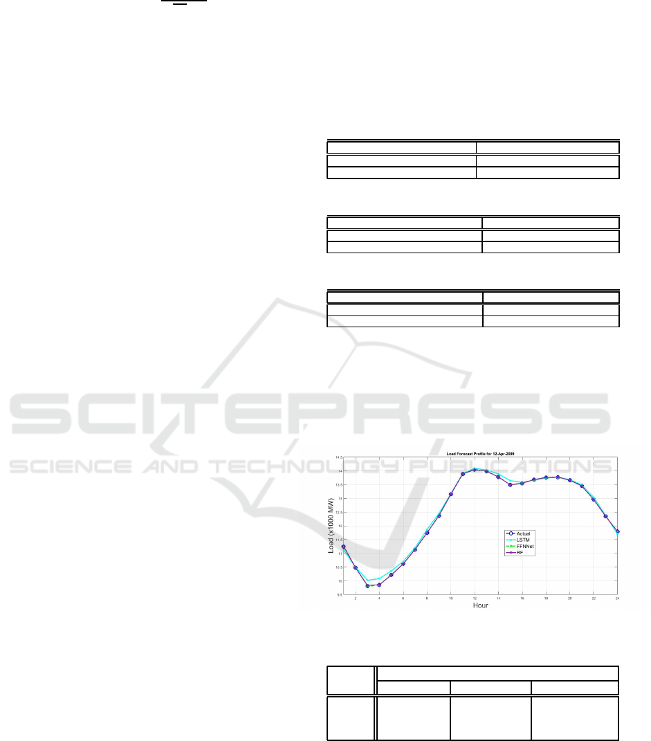
Figure 1: Day ahead hourly load forecast of Easter Day.
Table 4: MAPE, MAE and RMSE for Easter Day 2009.
Out of Sample
Model MAPE (%) MAE (MWh) RMSE (MWh)
LSTM 0.65 74.66 97.07
FFNN 6.24×10
−7
7.37×10
−5
8.68×10
−5
RF 0.045 5.20 7.03
The x-axis of the graph represents the hours of the
anomalous day and the y-axis represents the load de-
mand in megawatt. From the graphs and outlined in
the tables of Model evaluation metrics, the Feedfor-
ward Neural Network (FFNN) is a better fit to the data
followed by the Random Forest (RF) and last is the
Multivariate Short Term Load Forecasting Strategy: Application to Anomalous Days of ISO New England Data
299

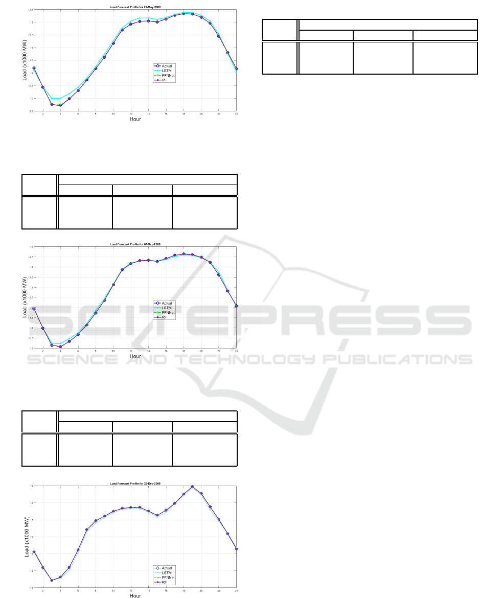
Figure 2: Day ahead hourly load forecast of Memorial Day
2009.
Table 5: MAPE, MAE and RMSE for Memorial Day 2009.
Out of Sample
Model MAPE (%) MAE (MWh) RMSE (MWh)
LSTM 0.89 101.27 117.19
FFNN 6.00 ×10
−7
6.52×10
−5
9.23×10
−5
RF 0.042 4.62 7.48
Figure 3: Day ahead hourly load forecast of Labour Day
2009.
Table 6: MAPE, MAE and RMSE for Labour Day 2009.
Out of Sample
Model MAPE (%) MAE (MWh) RMSE (MWh)
LSTM 0.48 56.42 72.78
FFNN 4.42 ×10
−7
5.51×10
−5
6.10×10
−5
RF 0.032 3.86 4.94
Figure 4: Day ahead hourly load forecast of Christmas Day
2009.
Table 7: MAPE, MAE and RMSE for Christmas Day 2009.
Out of Sample
Model MAPE (%) MAE (MWh) RMSE (MWh)
LSTM 0.52 85.27 95.61
FFNN 3.73×10
−7
6.17×10
−5
7.04×10
−5
RF 0.014 2.33 2.68
Long Short Term Memory (LSTM) Neural Network.
The MAPE, MAE and RMSE from Table 4 to Table
7 show that the FFNN has achieved the lowest errors
and hence the highest accuracy in predicting the load
profile of the selected anomalous days. The predicted
load demand for the FFNN model is very close to the
actual load. The performance of the FFNN model
implies that with proper data preprocessing and ex-
cellent hyperparameter optimization shows that the
FFNN is capable of approximating any measurable
function to any desired degree of accuracy. The prob-
lem of overfitting was avoided during training by the
use of MATLAB R2020b function TRAINBR which
uses Bayesian regularization and enhances general-
ization as well. As the second best performing model
the Random Forest is however the one most prefered
the reason being their flexibility which is suitable for
linear and non-linear relationships, they take into ac-
count interactions among predictors at different lev-
els, no assumption on the data are needed, they pro-
vide very accurate predictions as evident in this study
and their interpretability. As the least performing
model, the LSTM model howevercan be improved by
adding several LSTM layers, optimizing hyperparam-
eters such as Gradient Decay Factor and the Squared
Gradient Decay Factor of the Adam Optimizer
5 CONCLUSIONS
The paper presented three multivariate Bayesian Op-
timization (BO) based Random Forest (RF), Feed-
forward Neural Networks (FFNN) and Long Short-
term Memory (LSTM) neural network for day ahead
hourly load forecast of the anomalous days system
load of the ISO New England grid. The predictor vari-
ables were subjected to Multivariate Denoising us-
ing Wavelet and Principal Component Analysis. The
methodology followed shows that the Feedforward
Neural Networks achieved superior results. Also, the
main objective of this study was attained which was
to achieve a MAPE of less than 1% on the day ahead
hourly load forecast of the Anomalous Days of ISO
New England Grid Data. The major challenge going
forward is to apply our methodology to different grid
data sets.
NCTA 2021 - 13th International Conference on Neural Computation Theory and Applications
300

ACKNOWLEDGEMENTS
I would like to acknowledge the Faculty of Engineer-
ing and the Built Environment at the Durban Univer-
sity of Technology for their financial support.
REFERENCES
Aminghafari, M., Cheze, N., and Poggi, J.-M. (2006). Mul-
tivariate de-noising using wavelets and principal com-
ponent analysis. In Computational Statistics and Data
Analysis, 50, pp. 2381–2398. ELSEVIER.
Claesen, M. and Moor, B. D. (2015). Hyperparame-
ter search in machine learning. In arXiv preprint
arXiv:1502.02127. CORNELL UNIVERSITY.
Greff, K., Shrivastava, R. K., Koutnik, J., Steunebrink,
B. R., and Schmidhuber, J. (2017). Lstm: A search
space odyssey. In IEEE Transactions on Neural Net-
works and Learning Systems, vol. 28, issue 10, pp.
2222–2232. IEEEXplore.
He, F., Zhou, J., Feng, Z., Liu, G., and Yang, Y. (2019).
A hybrid short-term load forecasting model based on
variational mode decomposition and long short-term
memory networks considering relevant factors with
bayesian optimization algorithm. In Applied Energy,
237, pp. 103–116. SCIENCEDIRECT.
Hobbs, B. F., Jitprapaikulsarn, S., Konda, S., Chankong, V.,
Loparo, K. A., and Maratukulam, D. J. (1999). Analy-
sis of the value for unit commitment of improved load
forecasts. In IEEE Transactions on Power Systems,
vol. 14, no. 4, pp. 1342–1348. IEEEXplore.
Kandananond, K. (2011). Forecating electricity demand in
thailand with an artificial neural network approach. In
Energies, 4(8), 1246–1257. MDPI.
Kapoor, A. and Sharma, A. (2018). A comparison of short-
term load forecasting techniques. In 2018 IEEE In-
novative Smart Grid Technologies - Asia (ISGT Asia),
Singapore, pp. 1189–1194. UIASSIST.ORG.
Munem, M., Bashar, T. M. R., Roni, M. H., Shahriar,
M., Shawkat, T. B., and Rahaman, H. (2020). Elec-
tric power load forecasting based on multivariate long
short-term memory neural network using bayesian op-
timization. In 2020 IEEE Electric Power and Energy
Conference (EPEC), Edmonton, AB, Canada, pp. 1–6.
IEEEXplore.
Nti, I. K., Teimeh, M., Nyarko, O., and Adekoya, A. F.
(2020). Electricity load forecasting: A systematic re-
view. In Journal of Electrical Systems and Informa-
tion Technology 7, 13. Springer.
Rana, M. and Koprinska, I. (2016). Forecasting electricity
load with advanced wavelet neural networks. In Neu-
rocomputing, 182, pp. 118–132. ELSEVIER.
Raza, M. Q., Mithulananthan, N., Li, J., and Lee, K. Y.
(2020). Multivariate ensemble forecast framework for
demand prediction of anomalous days. In IEEE Trans-
actions on Sustainable Energy, vol. 11, no. 1, pp. 27–
36. IEEEXplore.
Sak, H., Senior, A., and Beaufays, F. (2014). Long short-
term memory recurrent neural network architectures
for large scale acoustic modeling. In In Proceed-
ings of the Annual Conference of International Speech
Communication Association (INTERSPEECH). RE-
SEARCHGOOGLE.
Son, H. and Kim, C. (2020). A deep learning approach
to forecasting monthly demand for residential-sector
electricity. In Sustainability, 12, 3103. MDPI.
Wang, J., Wang, J., Li, Y., Zhu, S., and Zhao, J. (2014).
Techniques of applying wavelet de-noising into a
combined model for short-term load forecasting. In
Electrical Power and Energy Systems, 62, pp. 816–
824. ELSEVIER.
Multivariate Short Term Load Forecasting Strategy: Application to Anomalous Days of ISO New England Data
301