Relaxed Dissimilarity-based Symbolic Histogram Variants for Granular

Graph Embedding

Luca Baldini

1 a

, Alessio Martino

2,3 b

and Antonello Rizzi

1 c

Department of Information Engineering, Electronics and Telecommunications, University of Rome “La Sapienza",

Via Eudossiana 18, 00184 Rome, Italy

Institute of Cognitive Sciences and Technologies (ISTC-CNR), Italian National Research Council,

Via San Martino della Battaglia 44, 00185 Rome, Italy

Department of Business and Management, LUISS University, Viale Romania 32, 00197 Rome, Italy

Keywords:

Structural Pattern Recognition, Supervised Learning, Embedding Spaces, Granular Computing, Graph Edit

Distances, Graph Embedding.

Abstract:

Graph embedding is an established and popular approach when designing graph-based pattern recognition

systems. Amongst the several strategies, in the last ten years, Granular Computing emerged as a promising

framework for structural pattern recognition. In the late 2000’s, symbolic histograms have been proposed as

the driving force in order to perform the graph embedding procedure by counting the number of times each

granule of information appears in the graph to be embedded. Similarly to a bag-of-words representation of

a text corpora, symbolic histograms have been originally conceived as integer-valued vectorial representation

of the graphs. In this paper, we propose six ‘relaxed’ versions of symbolic histograms, where the proper

dissimilarity values between the information granules and the constituent parts of the graph to be embedded

are taken into account, information which is discarded in the original symbolic histogram formulation due

to the hard-limited nature of the counting procedure. Experimental results on six open-access datasets of

fully-labelled graphs show comparable performance in terms of classiﬁcation accuracy with respect to the

original symbolic histograms (average accuracy shift ranging from -7% to +2%), counterbalanced by a great

improvement in terms of number of resulting information granules, hence number of features in the embedding

space (up to 75% less features, on average).

1 INTRODUCTION

In the last two decades, we witnessed a growing in-

terest of the scientiﬁc community in applying pat-

tern recognition (and related ﬁelds) techniques to the

domain of graph data structures. This interest can

be naturally explained by the representation power

conveyed by the semantic and topological descrip-

tion that graph domain offers in describing processes

where objects or entities interact together. In fact,

structured data such as graphs are largely used to

model complex phenomena in different application

ﬁelds such as economic markets, human social inter-

actions, immune systems, disease diffusion and gen-

erally in situations where parts of the system under

investigation are connected together in a network rep-

https://orcid.org/0000-0003-4391-2598

https://orcid.org/0000-0003-1730-5436

https://orcid.org/0000-0001-8244-0015

resented as a graph.

On the other hand, the deployment of pattern

recognition techniques in graph domain is a non-

trivial operation due its implicit structured and com-

binatorial nature. Compared to geometric spaces

such as the Euclidean one, basic algebraic operations

like the computation of similarity or dissimilarity be-

tween two graphs are not naturally deﬁned. Further-

more, vector data are static objects with predeﬁned

length, whilst different patterns in a set of graphs

can show different sizes in terms of number of nodes

and/or edges, posing additional limitations in utiliz-

ing a plethora of well-known statistical learning algo-

rithms (Bunke, 2003).

It is possible to spot three main approaches in the

current literature for dealing with the limitations im-

posed by the non-geometrical nature of the graph do-

main. The most intuitive and natural approach con-

sists in deﬁning an ad-hoc dissimilarity measure di-

Baldini, L., Martino, A. and Rizzi, A.

Relaxed Dissimilarity-based Symbolic Histogram Variants for Granular Graph Embedding.

DOI: 10.5220/0010652500003063

In Proceedings of the 13th International Joint Conference on Computational Intelligence (IJCCI 2021), pages 221-235

ISBN: 978-989-758-534-0; ISSN: 2184-3236

221

rectly in the graph domain, notably Graph Edit Dis-

tances (GED) (Bunke and Jiang, 2000; Riesen et al.,

2010; Bunke and Allermann, 1983). In the latest

decades, kernel methods have been deeply studied

as a valid approach for combining pattern recogni-

tion and graph domain (Ghosh et al., 2018; Kriege

et al., 2020). Given a kernel function κ : G × G

where G is the graph domain, kernel methods mea-

sure the pairwise similarities between graphs. When

the resulting kernel matrix K (i.e., the matrix con-

taining all the pairwise kernel evaluations between

the available graphs) is positive (semi)deﬁnite, κ is

valid dot product in an implicit Hilbert space. Op-

posite to kernel methods, graph embedding proce-

dures explicitly map graphs into a geometric embed-

ding space thanks to a suitable embedding function

Φ : G → X , where X ⊆ R

. This approach results

very ﬂexible since it enables the use of all the algo-

rithmic frameworks available in the ﬁeld of pattern

recognition. The main challenge posed by graph em-

bedding approaches is to correctly design a Φ func-

tion able to keep topological and semantic properties

of the original domain intact in the target domain. For

this reason, several mapping functions have been pro-

posed and applied in different application domains.

A straightforward method consists in manually col-

lect n relevant descriptive numerical features of the

graph into a n-length real-valued vector. Such ap-

proach can be tedious and requires a deep (and often

not available) knowledge of the underlying process.

In (Bunke and Riesen, 2008), the authors introduced

a graph embedding procedure based on dissimilarity

representation (P˛ekalska and Duin, 2005; Duin and

P˛ekalska, 2012). Given a set R of n prototype graphs

extracted from the training data and a graph G to be

embedded, the vector representation of G can be ex-

pressed as an n-length vector whose i

component is

deﬁned as d (p

,G), where p

∈ R and d : G × G is

a suitable dissimilarity measure. Major drawbacks of

this procedure are the computational cost needed for

evaluating d(·,·) between large graphs and/or large

datasets and the choice of enough informative pro-

totypes to populate R (P˛ekalska et al., 2006). An-

other interesting human inspired paradigm known as

Granular Computing (GrC) (Zadeh, 1997; Bargiela

and Pedrycz, 2003; Pedrycz, 2001) can be exploited

for graph embedding scope. A GrC approach con-

sists in extracting relevant information (known as in-

formation granules) by observing the problem at dif-

ferent levels of abstraction. In (Bianchi et al., 2014),

GrC has been employed for extracting automatically

relevant prototype subgraphs in conjunction with the

symbolic histogram representation for performing the

embedding procedure (Del Vescovo and Rizzi, 2007a;

Del Vescovo and Rizzi, 2007b). In particular, from

the symbolic histogram perspective, the i

compo-

nent of the embedded graph G is obtained by count-

ing the occurrences of i

relevant substructure (i.e.,

the granule extracted with a suitable granulation pro-

cedure) in G. The process of occurrences counting

is accomplished by an hard-limiting function which

triggers a counter whether the dissimilarity measure

between the speciﬁc prototype and a subgraph g ∈ G

is below a given threshold.

In this paper, we investigate a novel approach

based on symbolic histograms for granular graph em-

bedding. In particular, we ‘relax’ the evaluation of

the occurrences for the symbolic histogram in favour

of three different types of functions, that is, instead of

relying on counting the number of occurrences (i.e.,

an integer-valued embedding vector), we take into

consideration the proper dissimilarity values when

searching for granules occurrences within the graph

to be embedded, following the rationale behind the

aforementioned dissimilarity space embedding.

The remainder of the paper is structured as fol-

lows: in Section 2 we describe the GrC-based classi-

ﬁcation system, along with the original symbolic his-

tograms deﬁnition; Section 3 contains the main nov-

elty of the paper, as we describe the six ‘relaxed’ sym-

bolic histograms variants; Section 4 regards the com-

putational experiments, including an exhaustive com-

parison against state-of-the-art techniques. Finally,

Section 5 concludes the paper. The paper also fea-

tures an Appendix in which we give an example of

how GrC-based pattern recognition systems allow a

certain degree of interpretability by analyzing the re-

sulting granules of information.

2 GRANULAR GRAPH

EMBEDDING WITH

SYMBOLIC HISTOGRAMS

In this section, we describe the procedure that allows

the embedding and classiﬁcation of a set of graphs

according to the GrC paradigm. The core idea be-

hind this method is to synthesize an alphabet of sym-

bols A = {s

,...,s

}, namely the set of meaningful

and relevant subgraphs extracted from the training

set under analysis by following a granular approach.

The symbols, i.e. granules of information, emerge

thanks to a granulation procedure based on the Ba-

sic Sequential Algorithmic Scheme (BSAS) free clus-

tering method (Theodoridis and Koutroumbas, 2008),

driven by a resolution parameter θ which determines

the granularity level of observation. Finally, the gen-

NCTA 2021 - 13th International Conference on Neural Computation Theory and Applications

222

erated alphabet A is employed for building the sym-

bolic histogram of each graph, hence moving the clas-

siﬁcation problem towards a metric space where any

statistical classiﬁer can be employed. In the seminal

paper (Bianchi et al., 2014), this approach has been

successfully exploited for building a graph classiﬁca-

tion system named GRALG.

2.1 Substructures Extraction

Starting from the training set S

(tr)

, this block extracts

a set of subgraphs S

(tr)

. The design of this block is

crucial for two different aspects that can undermine

the entire embedding procedure. From a memory

footprint point of view, an exhaustive extraction of all

the subgraphs in S

(tr)

can be unfeasible. In fact, the

number of subgraphs that can be extracted from a sin-

gle graph grows combinatorially with the number of

its nodes. This poses a serious limitation to the usabil-

ity of this approach, constricting the application ﬁeld

to problems involving graphs of small size. Addition-

ally, the computational cost of the following blocks,

in particular the granulation procedure, are strongly

inﬂuenced by the number of elements in S

(tr)

, pos-

sibly making the entire graph embedding procedure

unfeasible. The second aspects regards the choice

of the desired topology of the subgraphs to be ex-

tracted (e.g., cliques, paths, stars and the like). Even

though this point can give ﬂexibility to our approach,

the selection of an appropriate traversal algorithm is

not trivial and likely inﬂuences the performance of a

graph classiﬁcation system driven by ﬁnding mean-

ingful subgraphs for graph embedding purposes (like

the one we present in this work) since the topological

properties of the original graphs must be reﬂected in

the subgraphs to be extracted. In this work, we use the

stratiﬁed stochastic extraction procedure proposed in

(Baldini et al., 2021) in order to limit the cardinality

of S

(tr)

to a user-deﬁned value W . The procedure goes

as follows:

1. For a given problem-related class, say the i

, ﬁnd

the number of subgraphs to be extracted as f =

W ·

(tr,i)

|S|

, where S

(tr,i)

denotes the subset of S

(tr)

containing only patterns belonging to class i

(a) A single graph G is extracted uniformly at ran-

dom from S

(tr,i)

(b) The selected graph G is visited using one of the

many traversing strategies available in the com-

puter science and graph theory communities–

such as Breath First Search (BFS), Depth First

Search (DFS) and random walks–until a ﬁxed

number of nodes V are visited

ing subgraph g and collected into S

(tr,i)

(d) The procedure goes back to 1a until the cardi-

nality of S

(tr,i)

has reached f

2. The procedure goes back to 1 until all classes are

considered.

The rationale behind the stratiﬁed approach is that

the bucket of subgraphs S

(tr)

is actually a bucket-of-

buckets S

(tr)

= {S

(tr,1)

,...,S

(tr,c)

}, with c being the

number of classes, in such a way that the i

bucket

only contains subgraphs extracted from patterns be-

longing to class i. This assures that, if compared to

a purely uniform random extraction (Baldini. et al.,

2019), all classes are represented in the bucket, with

a stratiﬁed number of subgraphs that scales according

to the frequency of the class itself (see Step #1), to

ensure fairness in the distribution.

2.2 Granulation Method for Alphabet

Synthesis

In this subsection, we give a formal description of

the process that synthesizes the alphabet A. In the

spirit of GrC, each symbol s

∈ A is an highly infor-

mative mathematical entity following the principle of

justiﬁable granularity related to the speciﬁc level of

abstraction at which the problem has been observed

(Pedrycz and Homenda, 2013). In the literature, many

authors have given several different deﬁnitions of in-

formation granule: fuzzy sets, rough sets and shad-

owed sets (Pedrycz et al., 2015) are just few exam-

ples on how granules can be practically formalized.

In our work, we follow a clustering-based approach

(Wang et al., 2016) for formally deﬁning a granule

of information. As anticipated in Section 2, the core

of the granulation procedure is the BSAS algorithm

working directly on the set of subgraphs S

(tr)

. It re-

lies on four fundamental actors: a threshold of in-

clusion θ, a clustering representative g

∗

, a dissimi-

larity measure d : G × G → R and a threshold Q of

maximum allowed number of clusters. By varying θ,

the clusters resolution will change accordingly, effec-

tively impacting on the granularity level. Thus, we

generate a set of partitions P = {P

,...,P

}, where

partition P

collects each cluster C emerged by im-

posing θ

as the resolution value. In order to account

for only well-formed clusters as candidate informa-

tion granules, we deﬁne the following cluster quality

index F (C, ρ) ∈ [0,1] (the lower is better):

F (C,ρ) = ρ · Ψ(C) + (1 − ρ) · Ω (C) (1)

as the linear convex combination between Ψ (C) and

Ω(C), respectively compactness and cardinality of

Relaxed Dissimilarity-based Symbolic Histogram Variants for Granular Graph Embedding

223

cluster C, weighted by a trade-off parameter ρ ∈ [0, 1]:

Ψ(C) =

|C − 1|

∑

g∈C

d (g

∗

,g) (2)

Ω(C) = 1 −

|C|

(tr)

(3)

In this work, we assume g

∗

be the MinSOD

(Del Vescovo et al., 2014; Martino et al., 2019b) ele-

ment of C, that is the graph that minimizes the pair-

wise sum of distances among all patterns in the clus-

ter. Clearly, the dissimilarity measure d must be tai-

lored to the input space under analysis (i.e., the graph

domain): our choice felt on a weighted GED-based

heuristics named node-Best Match First (nBMF). Full

details on nBMF, along with detailed pseudocodes,

can be found in (Baldini. et al., 2019; Martino and

Rizzi, 2021).

Finally, each cluster proves its validity by compar-

ing its own quality F (C) with a threshold τ ∈ [0, 1].

The MinSoDs of the surviving clusters are then col-

lected together in the alphabet A.

Recalling that S

(tr)

is actually a set-of-sets, the

above procedure is independently evaluated on each

class-related bucket S

(tr,i)

i=1

: this means that c class-

aware alphabets A

(i)

i=1

are returned, hence the over-

all alphabet simply reads as the concatenation of the

class-related alphabets A = ∪

i=1

(i)

2.3 Embedding with Symbolic

Histograms

In this block, the embedding function Φ : G → X

is implemented by following the symbolic histogram

paradigm (Del Vescovo and Rizzi, 2007b). This

method allows the embedding of a graph G into a fea-

ture space X according to two core sets: the ﬁrst is a

collection of prototype substructures that, in our case,

coincides with the alphabet A obtained in Section 2.2;

the second G

exp

is the set of subgraphs that compose

G. In other words, G

exp

= {g

,. .. , g

} is a (possi-

bly non-exhaustive) decomposition of the graph G in

k atomic units. The symbolic histogram h

is then

deﬁned as:

= [occ(s

exp

),. .. , occ (s

exp

)] (4)

By observing Eq. (4), we can see that h

is an integer-

valued vector with n components, where n = |A|. The

process of counting occurrences of a symbol s

∈ A in

exp

is performed by the function occ : A × G → N,

deﬁned as follows:

occ(s

exp

) =

∑

g∈G

exp

Γ(s

,g) (5)

In Eq. (5), Γ is a function that deﬁnes whether a sym-

bol s

can be matched with a subgraph g ∈ G

exp

. Exact

match between two graphs (also known as graph or

subgraph isomorphism) is often an unpractical opera-

tion for its hardness from a computational complexity

point of view, especially when nodes and edges are

equipped with real-valued vectors or even with cus-

tom data structures (Emmert-Streib et al., 2016). In

order to account for inexactness in the matching pro-

cedure, Γ evaluates the degree of dissimilarity d(s

,g)

between s

and g, then it triggers the counter (i.e., a

match is considered a hit) only if this value does not

exceed a symbol-dependent threshold ζ

Γ(s

,g) =

(

1 if d(s

,g) ≤ ζ

0 otherwise

(6)

2.4 Alphabet Optimization

After having synthesized a candidate alphabet A,

each graph from the dataset at hand can be embedded

toward the resulting embedding space X ⊆ R

. A nat-

ural question that arise is how to determine the quality

of this embedding space in order to evaluate the good-

ness of A. A possible solution already explored in

GRALG consists in training a classiﬁer H in the em-

bedding space and evaluating a performance measure

π : X → R of H in classifying a validation set. Then,

π can be interpreted as a critic of H about the embed-

ding space X . In order to automatize the search for

a suitable and informative alphabet, an evolutionary

optimization phase (driven, for example, by a differ-

ential evolution (Storn and Price, 1997)) whose ﬁtness

function relies on π can be employed, aiming at syn-

thesizing ever-improving alphabets.

The genetic code of each individual,

summarized in Eq. (7), contains w =

node

ins

node

del

node

sub

edge

ins

edge

del

edge

sub

} ∈ [0,1]

which are the nodes and edges insertion, deletion,

substitution weights for the weighted GED and

γ, the set of parameters driving nodes and edges

dissimilarity measures (if applicable). Additionally,

the procedure optimizes the relevant parameters for

the granulation procedure, namely the maximum

number of clusters allowed for BSAS Q ∈ [1,Q

max

the quality threshold τ ∈ [0,1] for promoting symbols

to the alphabet and the compactness-vs-cardinality

trade-off parameter ρ ∈ [0,1].

[w γ

γ Q τ ρ] (7)

The objective function J

, to be minimized, is deﬁned

as follows:

= α · (1 − π) + (1 − α) ·

|A|

(tr)

(8)

NCTA 2021 - 13th International Conference on Neural Computation Theory and Applications

224

Thus, Eq. (8) can be read as a linear convex combina-

tion between the performance π (leftmost term) and

the penalty (rightmost term), with the latter aiming at

fostering sparse alphabets according to a user-deﬁned

trade-off parameter α ∈ [0,1].

More in detail, each individual from the evolving

population reads S

(tr)

(the set of subgraphs extracted

from the training set), S

(tr)

(the training set), S

(vs)

(the validation set) and exploits Q, τ and ρ for driv-

ing the granulation procedure which, in turn, relies on

the nBMF dissimilarity measure driven by w and γ

γ (if

applicable). As the alphabet A is returned by the gran-

ulation procedure (Section 2.2), the embedding takes

place (Section 2.3). Therefore, the individual builds

two instance matrices, namely H

(tr)

and H

(vs)

, respec-

tively an |S

(tr)

|×n and |S

(vs)

|×n matrix which see the

symbolic histograms of the training set and validation

set organized as rows. The performance π ∈ [0, 1] is

chosen as the classiﬁcation accuracy obtained by H

trained with H

(tr)

in classifying H

(vs)

Once the evolutionary strategy is completed, the

optimal alphabet

A is retained together with the opti-

mal genetic code which leads to the synthesis of

(tr)

(vs)

, respectively the vector representation of S

(tr)

and S

(vs)

obtained with

2.5 Feature Selection and Test Phase

It is not rare that after the alphabet optimization de-

scribed in the previous section, the cardinality of the

optimal alphabet set ˜n = |

A| can be very large, that is

A may contains a large number of symbols and thus

spanning vectors in high-dimensional spaces. There

are several problems that can arise and negatively

impact the performances of a classiﬁcation system,

including the curse of dimensionality (Tang et al.,

2014), longer training and testing times, deteriorated

model interpretability (Martino et al., 2020). For this

reason, a feature selection phase should be applied to

A in order to remove uninformative, redundant and in

general not necessary symbols for the classiﬁcation

task. A wrapper approach based on an evolutionary

algorithm has been designed for this purpose, where

the genetic code of each individual is a binary mask

m ∈ [0,1]

˜n

which allows the selection of a subset of

features. Hence, each individual:

1. reads

(tr)

and

(vs)

2. according to the 0’s in m, the corresponding

columns of

(tr)

and

(vs)

are removed, lead-

ing to projected matrices

0(tr)

∈ R

(tr)

|×n

and

0(vs)

∈ R

(vs)

|×n

where n

∑

˜n

i=1

3. a classiﬁer H is trained on

0(tr)

and its own per-

formance measure ω is computed as the misclas-

siﬁcation rate on

0(vs)

The objective function (to be minimized) is then de-

ﬁned as:

= (1 − λ) · ω + λ ·

˜n

(9)

which, as in the case of Eq. (8), reads as a convex

linear combination between the error rate on the val-

idation set (leftmost term) and the ratio of selected

symbols (rightmost term), weighted by a user-deﬁned

trade-off parameter λ ∈ [0,1].

Once the optimization is completed, the optimal

mask m

∗

is retained with H

∗(tr)

∈ R

(tr)

|×n

∗

, H

∗(vs)

∈

(vs)

|×n

∗

as well, where n

∗

∑

˜n

i=1

∗

. Accordingly,

the optimal alphabet A

∗

⊂

A is created by selecting

the features indicated by the 1’s in m

∗

The reduced alphabet A

∗

is the main actor when it

comes to address the generalization capabilities of the

whole system with a set of test data S

(ts)

. In fact, S

(ts)

is embedded thanks to A

∗

, hence returning H

∗(ts)

∈

(ts)

|×n

∗

, then the classiﬁer H is trained on H

∗(tr)

and ﬁnally tested on H

∗(ts)

3 RELAXED SYMBOLIC

HISTOGRAMS

From Section 2.3, let us recall the original symbolic

histogram. In short, it aims at representing the graph

to be embedded as a vector collecting (in the i

po-

sition) the number of occurrences of the i

symbol

from the alphabet A within the graph to be embedded

G, with the latter being properly decomposed (G

exp

)

to facilitate the search-and-matching procedure. It is

clear that the original symbolic histogram reads as

an integer-valued vector, where the proper symbol-

to-subgraphs dissimilarity values (i.e., d(s

,g) in Eq.

(6)) are not taken into account. Inspired by dissimi-

larity spaces (Section 1), where the dissimilarity value

amongst data is the core of the embedding procedure,

here below we present six different strategies in order

to populate the symbolic histogram, while at the same

time taking into account the dissimilarities between

symbols in the alphabet and the constituent parts of

the graph to be embedded.

3.1 Sum

The sum strategy aims at collecting, in the i

posi-

tion of the symbolic histogram, the sum of distances

between the i

symbol in the alphabet and the con-

stituent parts of the graph to be embedded. Formally,

= [sum(s

exp

),. .. , sum (s

exp

)] (10)

Relaxed Dissimilarity-based Symbolic Histogram Variants for Granular Graph Embedding

225

where the sum : A × G → R operator reads as

sum(s

exp

) =

∑

g∈G

exp

d(s

,g) (11)

3.2 Mean

The sum strategy is characterized by a couple of

caveats: a) dissimilarity values are summed up re-

gardless of their magnitude, b) the number of dissim-

ilarities that are summed up is not taken into account.

Especially in light of the second caveat, the mean

strategy accounts for the mean of distances between

the i

symbol in the alphabet and the constituent parts

of the graph to be embedded. Formally,

= [mean(s

exp

),. .. , mean (s

exp

)] (12)

where the mean : A × G → R operator reads as

mean(s

exp

) =

exp

∑

g∈G

exp

d(s

,g) (13)

It is worth noting that |G

exp

| varies on a graph-based

fashion (i.e., each symbolic histogram has its own

scaling factor as it depends on the graph G to be em-

bedded) and it is not equivalent to a constant scaling

of all symbolic histograms.

3.3 Median

It is well known that outliers might have a non-

negligible impact on the mean of a set of scalar values.

In our case, this reﬂects on very high or very low dis-

similarities that might skew the mean value. In order

to mitigate this effect, a more robust statistic based on

the median value is considered. Formally,

= [median (s

exp

),. .. , median (s

exp

)] (14)

where the median : A × G → R operator reads as

median(s

,g) =







exp

if |G

exp

| is even

exp

|−1

exp

|+1

if |G

exp

| is odd

(15)

and d ∈ R

1×|G

exp

is a vector that collects the pairwise

dissimilarities between s

and all items in g ∈ G

exp

sorted in ascending order.

3.4 Thresholded-sum

The three strategies discussed so far in Sections 3.1–

3.3 aim at aggregating, according to different oper-

ators, the pairwise symbol-to-subgraphs dissimilari-

ties for populating a given entry of the symbolic his-

togram. Yet, as introduced in Section 3.2, all dis-

similarities (regardless of their magnitude) are enti-

tled to contribute to a given entry of the symbolic his-

togram vector. Taking inspiration from the original

symbolic histogram (Section 2.3), we let dissimilari-

ties contribute to a given operator if and only if their

magnitude is below a given threshold.

As the sum operator is concerned, in Eq. (10), the

sum(·,·) operator, formerly Eq. (11), is replaced by

the following thresholded sum (or, for short, t-sum :

A × G → R) operator

t-sum(s

exp

) =

∑

g∈G

exp

d(s

,g)≤ζ

d(s

,g) (16)

where, recall, ζ

is a symbol-aware inclusion thresh-

old.

3.5 Thresholded-mean

The thresholded mean follows the same rationale be-

hind t-sum(·,·): only dissimilarities below a given

threshold are entitled to contribute to the mean value

for populating the symbolic histogram entries. That

is, the mean(·, ·) operator deﬁned in Eq. (13) to be

plugged into the symbolic histogram (see Eq. (12))

is replaced by the following thresholded mean (or, for

short, t-mean : A × G → R) operator

t-mean(s

exp

) =

∑

g∈G

exp

d(s

,g)≤ζ

d(s

,g)

|{g : d(s

,g) ≤ ζ

,∀g ∈ G

exp

(17)

3.6 Thresholded-median

Finally, the thresholded median (or, for short,

t-median : A × G → R) reads as the median(·,·) op-

erator in Eq. (15). The major difference is that the

(sorted) vector d will only contain dissimilarities be-

low the symbol-related thresholds ζ

4 TESTS AND RESULTS

4.1 Datasets Description

In order to test the proposed algorithm and the dif-

ferent embedding strategies, the following six open-

access datasets from the IAM Repository (Riesen and

Bunke, 2008) are considered:

AIDS: The AIDS dataset is composed by graphs rep-

resenting molecular compounds showing activity

or not against HIV. Molecules are converted into

graphs by representing atoms as nodes and the co-

valent bonds as edges. Nodes are labeled with

the number of the corresponding chemical sym-

bol and edges by the valence of the linkage.

NCTA 2021 - 13th International Conference on Neural Computation Theory and Applications

226

GREC: The GREC dataset consists of graphs repre-

senting symbols from architectural and electronic

drawings. Drawings have been pre-processed and

ending points, circles, corners and intersections

are considered as nodes labelled with their posi-

tion and type. Edges connecting such nodes are

equipped with a hierarchical data structure that

identiﬁes the type of connection and its charac-

teristics.

Letter: The Letter datasets involve graphs that rep-

resent distorted letter drawings. Amongst the

capital letters of the Roman alphabet, 15 have

been selected due to them being representable

by straight lines only. Drawings are then con-

verted into graphs by considering lines as edges

and ending points as nodes. Nodes are labelled

with a 2-dimensional vector indicating their po-

sition, whereas edges are unlabelled. Three dif-

ferent amount of distortion (Low, Medium, High)

account for three different datasets, hereinafter re-

ferred to as Letter-L, Letter-M and Letter-H, re-

spectively.

Mutagenicity: The Mutagenicity dataset is com-

posed by graphs representing molecular com-

pounds showing mutagenicity properties or not.

Similar to the AIDS dataset, nodes correspond to

atoms (labelled with their chemical symbol) and

edges are labelled with the valence of the linkage.

In Table 1 we show some basic statistics about the six

datasets. As the nodes and edges dissimilarities are

concerned, all of them are customized according to

the nodes and edges attributes for each dataset. GREC

is the only dataset for which the dissimilarity mea-

sures between nodes and edges are parametric them-

selves: such values populate γ

γ which shall be opti-

mized, as described in Section 2.4. Full details on the

dissimilarity measures for AIDS, Letter and GREC

can be found in (Martino and Rizzi, 2021) and (Bal-

dini et al., 2021). For Mutagenicity, as instead, the

dissimilarity measures between nodes and edges are

plain non-parametric simple matching between their

respective labels.

4.2 Comparison amongst Embedding

Strategies

The algorithm parameters are set as follows:

• a simple random walk is employed as graph

traversing strategy for mining subgraphs of maxi-

mum order V = 5 for the extraction phase (i.e., for

populating S

(tr)

))

In our previous work (Baldini. et al., 2019), we wit-

• a modiﬁed BFS

is employed for extracting sub-

graphs for the embedding phase (i.e., for building

exp

)

• W = 10%, 30%, 50% of |S

(tr)

max

|, with the latter be-

ing the maximum number of subgraphs of max-

imum order V = 5 attainable from the training

graphs

(i.e., an exhaustive extraction)

• Q

max

= 500/c, where c is the (dataset-dependent)

number of classes

• maximum number of 20 generations for both dif-

ferential evolution stages (alphabet optimization

and feature selection)

• 20 individuals for the population of the ﬁrst dif-

ferential evolution (alphabet optimization)

• 100 individuals for the population of the second

differential evolution (feature selection)

• α = 0.9 in the ﬁtness function J

of the ﬁrst dif-

ferential evolution (major weight to performance)

• λ = 0.1 in the ﬁtness function J

of the second dif-

ferential evolution (major weight to performance)

• K-Nearest Neighbours with K = 5 as classiﬁca-

tion system H

• ζ

= 1.1 · Ψ (C

) as (cluster-dependent) tolerance

value for the symbolic histograms evaluation.

In Figures 1, 2 and 3, we report the results obtained

by equipping the GRALG classiﬁcation system pre-

sented in Section 2 with the six different symbolic

histograms-inspired embedding methods as described

in Section 3. Each ﬁgure corresponds to either one of

the three subsampling rates W in order to address the

performances of the system as a function of the can-

didate number of subgraphs for the granulation phase.

In order to account for the stochastic nature of the al-

gorithm, results in the following have been averaged

across 10 different runs. We explored the efﬁciency

of our approach under three different point of views,

i.e. the classiﬁer performance measured on the test set

(ts)

and the cardinality of the alphabet before (|

A|)

nessed that there is no clear winner between BFS or DFS

in terms of performances and/or running times, so the ratio-

nale behind choosing random walks is that there exist the

possibility of having both star-like and path-like subgraphs

in S

(tr)

As proposed in (Baldini. et al., 2019), we use BFS to

extract subgraphs in such a way that already-visited nodes

do not appear as root nodes for following traversals: this

ensures a complete coverage of the graph to be embedded

whilst, at the same time, keeping a low number of resulting

subgraphs.

AIDS: 27589; GREC: 21009; Letter-L: 7975; Letter-

M: 8217; Letter-H: 12603; Mutagenicity: 449519.

Relaxed Dissimilarity-based Symbolic Histogram Variants for Granular Graph Embedding

227

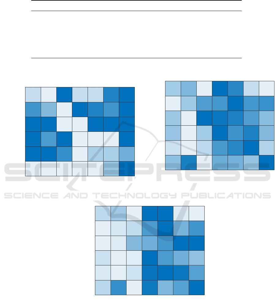
Table 1: Statistics of the considered datasets: number of graphs in training, validation and test set (|S

(tr)

|, |S

(vs)

|, |S

(ts)

|),

number of classes (c) and type of nodes and edges labels. Adapted from (Riesen and Bunke, 2008).

Dataset |S

(tr)

| |S

(vs)

| |S

(ts)

| c Node Labels Edge Labels

AIDS 250 250 1500 2 string + integer + R

integer

†

GREC 286 286 528 22 string + R

tuple

Letter-L 750 750 750 15 R

none

Letter-M 750 750 750 15 R

none

Letter-H 750 750 750 15 R

none

Mutagenicity 1500 500 2337 2 string integer

†

In our experiments, by following (Bianchi et al., 2014), the edge label has been dis-

carded.

Mean

Median

Sum

t-Mean

t-Median

t-Sum

Original

AIDS

GREC

Letter-L

Letter-M

Letter-H

Mutagenicity

0.93

0.81

0.66

0.92

0.79

0.91

0.66

0.76

0.96

0.66

0.93

0.96

0.89

0.87

0.66

0.93

0.89

0.88

0.66

0.81

0.89

0.88

0.67

0.89

0.97

0.92

0.91

0.97

0.91

0.99

0.92

0.9

0.83 0.82

0.97

0.98

0.97

0.99

0.83

0.97

0.92

0.69

(a) Accuracy on the Test Set.

Mean

Median

Sum

t-Mean

t-Median

t-Sum

Original

AIDS

GREC

Letter-L

Letter-M

Letter-H

Mutagenicity

82.67

143

86.67

121

160.3

333.7

121

213

68.67

144.3

295.7

116.7

168.7

260

306

234.3

360

166

354.7

45.67

308.3

104

326.3

90.33

132

175

427

123.7

262.3

121

196.3

217.7

378.3

116

253

182

275.7

316

450.3

(b) Embedding space dimensionality before Feature Selec-

tion.

Mean

Median

Sum

t-Mean

t-Median

t-Sum

Original

AIDS

GREC

Letter-L

Letter-M

Letter-H

Mutagenicity

14.33

52.33

5.67

30.67

39.33

83.33

23.33

63.33

6.33

20.67

34.33

77.33

13.33

66.67

157

14.67 18

74.67

105.3

127

61.33

120

164.7

84.33

131.7

75.33

101.3

113.3

147

209.7

116.3

23.33

112

23.33

153

Figure 1: Results at 10% subsampling rate. Color maps are normalized row-wise (i.e., independently for each dataset), with

a white-to-blue range mapping smallest-to-largest values.

and after (|A

∗

|) the feature selection phase (see Sec-

tion 2.5). It is worth noting that the performances on

the test set are obtained by the classiﬁer H trained

with H

∗(tr)

. Recall from Section 2.5 that the vectorial

representation H

∗(ts)

of S

(ts)

is obtained thanks to the

selected embedding procedure using the optimized al-

phabet A

∗

By comparing Figures 1a, 2a and 3a it is pos-

NCTA 2021 - 13th International Conference on Neural Computation Theory and Applications

228

Mean

Median

Sum

t-Mean

t-Median

t-Sum

Original

AIDS

GREC

Letter-L

Letter-M

Letter-H

Mutagenicity

0.92

0.67

0.92

0.67

0.77

0.96

0.67

0.91

0.79

0.89

0.87

0.67

0.91

0.8

0.89

0.88

0.8

0.96

0.9

0.88 0.88

0.67

0.82

0.97

0.93

0.92

0.81

0.97

0.93

0.91

0.99

0.93

0.91

0.97 0.97

0.68

0.98

0.68

0.99

0.82

0.97

0.92

(a) Accuracy on the Test Set.

Mean

Median

Sum

t-Mean

t-Median

t-Sum

Original

AIDS

GREC

Letter-L

Letter-M

Letter-H

Mutagenicity

138.7

86.67

106.3

123.7

191.7

180.3

101.3

139.7

172.3

171

11.67

290.7

121.7

234.7

237.7

304.7

312.3

142.7

494

151

340.3

28.33

233.7

151.7

252

231.7

348.7

633.3 564.3

261

412

221.7

301

297

460.7

295.7

374.7

378.7

298.7

387.7

(b) Embedding space dimensionality before Feature Selec-

tion.

Mean

Median

Sum

t-Mean

t-Median

t-Sum

Original

AIDS

GREC

Letter-L

Letter-M

Letter-H

Mutagenicity

23.33

15.33

27.33

23.33

17.67

43.67

66.67

51.33

56 105.3

18.33

172.7

120.3

108.7

87.33

112.3

155.7

175 171.3

201.7

27.67

111.3

144

84.33

251

123.7

161.3

203

29.33

108.3

163.3

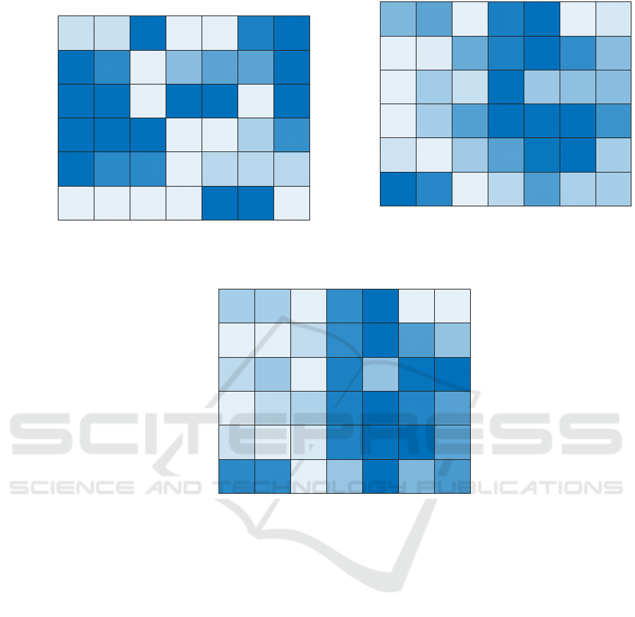
Figure 2: Results at 30% subsampling rate. Color map details in the caption of Figure 1.

sible to spot the differences in terms of accuracy.

The results depicted in the ﬁrst two columns (Mean

and Medium) witnessed that the selected embedding

methods are reaching comparable performances with

respect to the Original symbolic histogram method

equipped with the hard-limiting function regardless

of the number of candidate information granules W .

A note should be mentioned for AIDS, which is ar-

guably attaining lower level of performances (6~7

%) when compared with the Original column. On

the other hand, the remaining four approaches, i.e.

Sum, t-Mean, t-Median and t-Sum, show (on average)

worst performances when compared to Mean, Median

and Original. We again can observe an exception for

AIDS: when using the Sum aggregation operator, it

shows the highest result in terms of accuracy.

An interesting behaviour that emerge from the

tests regards the number of symbols that compose

the alphabets A

∗

and

A. With respect to thresh-

olded methods (t-Mean, t-Median, t-Sum and Orig-

inal), Mean, Median and Sum are by far producing

optimal alphabets with lower number of symbols, re-

gardless of W . This can be spotted by observing Fig-

ures 1c, 2c, 3c and their counterparts before the fea-

ture selection phase (Figures 1b, 2b, 3b), suggesting

that such reduction in terms of number of features is

not due to the feature selection phase but is a proper

characteristic of the aggregation function. With the

exception of Mutagenicity, all datasets show a clear-

cut difference in terms of alphabet cardinality when

not-thresholded methods are exploited. We advance

the hypothesis that by using hard-limiting functions

in the symbolic histograms, the resulting dynamic

of each vector component can be inﬂuenced by the

choice of the threshold. In fact, the set of parameters

(notably those related to the dissimilarity measure, i.e.

Relaxed Dissimilarity-based Symbolic Histogram Variants for Granular Graph Embedding

229

Mean

Median

Sum

t-Mean

t-Median

t-Sum

Original

AIDS

GREC

Letter-L

Letter-M

Letter-H

Mutagenicity

0.92

0.81

0.97

0.68

0.91

0.97

0.67

0.75

0.96

0.66

0.93

0.89

0.88

0.67

0.93

0.81

0.97

0.9

0.86

0.68

0.82

0.96

0.91

0.86

0.97

0.92

0.94

0.91

0.84

0.93

0.92

0.99

0.93

0.91

0.85

0.98

0.69

0.99

0.85

0.91

0.69

(a) Accuracy on the Test Set.

Mean

Median

Sum

t-Mean

t-Median

t-Sum

Original

AIDS

GREC

Letter-L

Letter-M

Letter-H

Mutagenicity

167.7

144.3

180

210.7

165

124.7

276.3

259

310.7

452.7

270.7

113.3

330.3

173.3

21.33

296.3

216

325.7

39.33

178.7

259

347

316.3

407.7

264

319

287

564.3

271.7

366

359

386.3

275.7

356

400.3

403.3

317.7

386.3

531.7

(b) Embedding space dimensionality before Feature Selec-

tion.

Mean

Median

Sum

t-Mean

t-Median

t-Sum

Original

AIDS

GREC

Letter-L

Letter-M

Letter-H

Mutagenicity

5.33

44.33

37.33

60.67

76.67

50.33

12.33

60.33

60.67

115.3

54.67

59.67

22.67

53.33

148.7

177.7

1.67

143.3

116.7

147

2.33

97.67

154.7

108.3

295.3

42.67

148.3

152.3

151.7

202

179

46.33

138

263.3

43.67

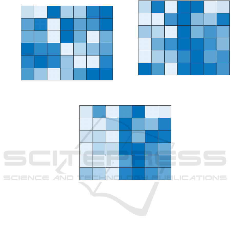
Figure 3: Results at 50% subsampling rate. Color map details in the caption of Figure 1.

w, γ

γ) explored by the evolutionary algorithm might

not be suitable enough for imposing an expressive dis-

similarity measure able to fairly compare the symbols

with the substructure set G

exp

. In this particular sit-

uation, most of the symbols would not be matched

with substructures in G

exp

, leading to an uninforma-

tive embedding space spanned by ﬂat vectors possibly

having many null components. On the other hand,

the evolutionary algorithm in the attempt to optimize

the error rate might be tempted to relieve this issue

by exploring granulation parameters (i.e., Q, τ and ρ)

which allow larger alphabets with higher chances of

scoring matches between symbols and the substruc-

tures of the graphs to be embedded. Clearly, this

situation does not hold in non-thresholded methods,

where each match counts (albeit proportionally to its

dissimilarity degree): in turn, this means that a given

symbol from the alphabet is (in very plain terms) ‘al-

ways found’ in the graph to be embedded which is

therefore completely explored during the embedding

procedure.

4.3 Comparison against

State-of-the-Art Techniques

In Section 4.2 we focused the computational results

on the comparison amongst the six different strate-

gies for populating the symbolic histograms presented

in Section 3. Hereinafter, we move the comparison

against other state-of-the-art techniques, summarized

in Table 2. Competitors span a variety of approaches

for graph classiﬁcation (as brieﬂy reviewed in Section

1), namely:

• classiﬁers working on the top of pure graph

matching similarities (Riesen and Bunke, 2008;

Riesen and Bunke, 2009a);

NCTA 2021 - 13th International Conference on Neural Computation Theory and Applications

230

• kernel methods (Da San Martino et al., 2016;

Martino and Rizzi, 2020);

• several embedding techniques (Riesen and Bunke,

2009b; Gibert et al., 2011), including GrC-based

(Martino et al., 2019a; Baldini. et al., 2019; Mar-

tino and Rizzi, 2021; Baldini et al., 2021) and

neural-based ones (Bacciu et al., 2018; Martineau

et al., 2020).

The accuracy of the last eight methods are obtained

from our own experiments. For the remaining com-

peting algorithms, we directly quote results from their

respective papers.

Clearly, GRALG also whether equipped with ‘re-

laxed’ symbolic histograms, is able to reach state-of-

the-art performances for 4 out of 6 datasets while,

at the same time, is able to return an interpretable

model: the same peculiarity only holds in other GrC-

based pattern recognition systems (namely (Martino

et al., 2019a; Baldini. et al., 2019; Martino and Rizzi,

2021; Baldini et al., 2021)), whilst it is well-known

that other learning paradigms, notably those based on

artiﬁcial neural networks (Xu et al., 2019), lack any

interpretation.

Speciﬁcally, for AIDS and Letter-H the perfor-

mance shift with respect to the most performing tech-

nique is below 1%; for Letter-L and Letter-M the gap

slightly increases to approximately 2%. Mutagenic-

ity and GREC are the only two datasets for which

the shift with respect to the most performing tech-

nique becomes larger: approximately 10% for the for-

mer and approximately 6% for the latter dataset, if we

omit the results obtained via cross-validation.

Table 2: Comparison against state of the art graph classiﬁcation system in terms of accuracy, expressed in percentage. Best

accuracy amongst all subsampling values have been reported for methods based on GRALG. A dash (-) indicates that a given

dataset has not been tested in the literature on the corresponding model.

Technique AIDS GREC Letter-L Letter-M Letter-H Mutagenicity Reference

Bipartite Graph Matching + K-NN - 86.3 91.1 77.6 61.6 - (Riesen and Bunke, 2009a)

Lipschitz Embedding + SVM 98.3 96.8 99.3 95.9 92.5 74.9 (Riesen and Bunke, 2009b)

Graph Edit Distance + K-NN 97.3 95.5 99.6 94 90 71.5 (Riesen and Bunke, 2008)

Graph of Words + K-NN - 97.5 98.8 - - - (Gibert et al., 2011)

Graph of Words + kPCA + K-NN - 97.1 97.6 - - - (Gibert et al., 2011)

Graph of Words + ICA + K-NN - 58.9 82.8 - - - (Gibert et al., 2011)

ODD ST

kernel 82.06* - - - - - (Da San Martino et al., 2016)

ODD ST

TANH

kernel 82.54* - - - - - (Da San Martino et al., 2016)

CGMM + linear SVM 84.16* - - - - - (Bacciu et al., 2018)

G-L-Perceptron - 70 95 64 70 - (Martineau et al., 2020)

G-M-Perceptron - 75 98 87 81 - (Martineau et al., 2020)

C-1NN - - 96 93 84 - (Martineau et al., 2020)

C-M-1NN - - 98 81 71 - (Martineau et al., 2020)

Hypergraph Embedding + SVM 99.3

†

- - - - 77.0

†

(Martino et al., 2019a)

RECTIFIER + K-NN 99.07 95.57 97.12 92.16 91.60 - (Martino and Rizzi, 2021)

Dual RECTIFIER + K-NN 99.13 96.61 96.40 93.04 91.31 - (Martino and Rizzi, 2021)

HCK Hypergraph kernel + SVM 89.5*

†

- - - - 73.3

†

(Martino and Rizzi, 2020)

WJK Hypergraph kernel + SVM 99.5*

†

- - - - 82

†

(Martino and Rizzi, 2020)

EK Hypergraph kernel + SVM 99.5*

†

- - - - 75.4

†

(Martino and Rizzi, 2020)

SEK Hypergraph kernel + SVM 99.6*

†

- - - - 75.3

†

(Martino and Rizzi, 2020)

GRALG (simple random walk)

original symbolic histogram

99.16 84.04 96.58 86.58 73.84 74.73 (Baldini. et al., 2019)

GRALG (stratiﬁed random walk)

original symbolic histogram

99 85 97 92 91 69

This work

also in (Baldini et al., 2021)

GRALG (stratiﬁed random walk)

sum symbolic histogram

99 77 96 93 91 67 This work

GRALG (stratiﬁed random walk)

mean symbolic histogram

93 82 97 94 92 68 This work

GRALG (stratiﬁed random walk)

median symbolic histogram

92 84 97 93 92 67 This work

GRALG (stratiﬁed random walk)

t-sum symbolic histogram

98 82 97 91 88 69 This work

GRALG (stratiﬁed random walk)

t-mean symbolic histogram

93 85 98 89 88 67 This work

GRALG (stratiﬁed random walk)

t-median symbolic histogram

93 82 97 90 88 68 This work

Results refer to cross-validation rather than a separate test set.

†

Only chemical symbol type (categorical) as node label. Edge labels are discarded.

Relaxed Dissimilarity-based Symbolic Histogram Variants for Granular Graph Embedding

231

5 CONCLUSIONS

In this paper, we proposed six ‘relaxed’ variants

of symbolic histograms for graph classiﬁcation pur-

poses. Inspired by the dissimilarity space embed-

ding, the ‘relaxed’ variants take into consideration the

proper magnitude of the dissimilarities when match-

ing the pivotal granules of information against the

constituent parts of the graphs to be embedded. Three

operators (mean, sum and median of distances) have

been proposed to aggregate such dissimilarity values,

with additional three variants which include a thresh-

olding stage in order to account only for similarities

that are ‘close enough’ with respect to the information

granule under analysis.

In order to test these variants against the original

symbolic histogram deﬁnition, we exploited a GrC-

based framework for graph classiﬁcation, namely

GRALG, and plugged the different symbolic his-

togram variants within the embedding module.

Six open-access datasets of fully labelled graphs

corroborate the effectiveness of the ‘relaxed’ variants.

Especially when the thresholding stage is not em-

ployed, the resulting set of pivotal symbols is dras-

tically reduced with respect to the thresholded vari-

ants (including the original symbolic histogram). In

conclusion, the non-thresholded mean and median

emerged as the most interesting operators in order to

populate the (relaxed) symbolic histogram since they

leaded to very small embedding spaces while, at the

same time, maintaining interesting performances in

terms of accuracy on the test set.

REFERENCES

Bacciu, D., Errica, F., and Micheli, A. (2018). Contextual

graph markov model: A deep and generative approach

to graph processing. In 35th International Conference

on Machine Learning, ICML 2018, volume 1, pages

495–504.

Baldini., L., Martino., A., and Rizzi., A. (2019). Stochas-

tic information granules extraction for graph embed-

ding and classiﬁcation. In Proceedings of the 11th

International Joint Conference on Computational In-

telligence - NCTA, (IJCCI 2019), pages 391–402. IN-

STICC, SciTePress.

Baldini, L., Martino, A., and Rizzi, A. (2021). Towards

a class-aware information granulation for graph em-

bedding and classiﬁcation. In Merelo, J. J., Garibaldi,

J., Linares-Barranco, A., Warwick, K., and Madani,

K., editors, Computational Intelligence: 11th Inter-

national Joint Conference, IJCCI 2019 Vienna, Aus-

tria, September 17–19, 2019, Revised Selected Pa-

pers. Springer International Publishing.

Bargiela, A. and Pedrycz, W. (2003). Granular comput-

ing: an introduction. Kluwer Academic Publishers,

Boston.

Bianchi, F. M., Livi, L., Rizzi, A., and Sadeghian, A.

(2014). A granular computing approach to the design

of optimized graph classiﬁcation systems. Soft Com-

puting, 18(2):393–412.

Bunke, H. (2003). Graph-based tools for data mining and

machine learning. In Perner, P. and Rosenfeld, A., ed-

itors, Machine Learning and Data Mining in Pattern

Recognition, pages 7–19, Berlin, Heidelberg. Springer

Berlin Heidelberg.

Bunke, H. and Allermann, G. (1983). Inexact graph match-

ing for structural pattern recognition. Pattern Recog-

nition Letters, 1(4):245 – 253.

Bunke, H. and Jiang, X. (2000). Graph matching and simi-

larity. In Teodorescu, H.-N., Mlynek, D., Kandel, A.,

and Zimmermann, H.-J., editors, Intelligent Systems

and Interfaces, pages 281–304. Springer US, Boston,

MA.

Bunke, H. and Riesen, K. (2008). Graph classiﬁcation based

on dissimilarity space embedding. In Joint IAPR

International Workshops on Statistical Techniques in

Pattern Recognition (SPR) and Structural and Syn-

tactic Pattern Recognition (SSPR), pages 996–1007.

Springer.

Da San Martino, G., Navarin, N., and Sperduti, A. (2016).

Ordered decompositional dag kernels enhancements.

Neurocomputing, 192:92 – 103.

Del Vescovo, G., Livi, L., Frattale Mascioli, F. M., and

Rizzi, A. (2014). On the problem of modeling struc-

tured data with the minsod representative. Interna-

tional Journal of Computer Theory and Engineering,

6(1):9.

Del Vescovo, G. and Rizzi, A. (2007a). Automatic classi-

ﬁcation of graphs by symbolic histograms. In 2007

IEEE International Conference on Granular Comput-

ing (GRC 2007), pages 410–410.

Del Vescovo, G. and Rizzi, A. (2007b). Online handwrit-

ing recognition by the symbolic histograms approach.

In 2007 IEEE International Conference on Granular

Computing (GRC 2007), pages 686–686. IEEE.

Duin, R. P. and P˛ekalska, E. (2012). The dissimilar-

ity space: Bridging structural and statistical pattern

recognition. Pattern Recognition Letters, 33(7):826–

832.

Emmert-Streib, F., Dehmer, M., and Shi, Y. (2016). Fifty

years of graph matching, network alignment and net-

work comparison. Information sciences, 346:180–

197.

Ghosh, S., Das, N., Gonçalves, T., Quaresma, P., and

Kundu, M. (2018). The journey of graph kernels

through two decades. Computer Science Review,

27:88–111.

Gibert, J., Valveny, E., and Bunke, H. (2011). Dimensional-

ity reduction for graph of words embedding. In Jiang,

X., Ferrer, M., and Torsello, A., editors, Graph-Based

Representations in Pattern Recognition, pages 22–31.

Springer Berlin Heidelberg, Berlin, Heidelberg.

NCTA 2021 - 13th International Conference on Neural Computation Theory and Applications

232

Kriege, N. M., Johansson, F. D., and Morris, C. (2020). A

survey on graph kernels. Applied Network Science,

5(1):6.

Martineau, M., Raveaux, R., Conte, D., and Venturini,

G. (2020). Learning error-correcting graph matching

with a multiclass neural network. Pattern Recognition

Letters, 134:68 – 76.

Martino, A., Frattale Mascioli, F. M., and Rizzi, A. (2020).

On the optimization of embedding spaces via infor-

mation granulation for pattern recognition. In 2020

International Joint Conference on Neural Networks

(IJCNN), pages 1–8.

Martino, A., Giuliani, A., and Rizzi, A. (2019a). (hy-

per)graph embedding and classiﬁcation via simplicial

complexes. Algorithms, 12(11).

Martino, A. and Rizzi, A. (2020). (hyper)graph kernels over

simplicial complexes. Entropy, 22(10).

Martino, A. and Rizzi, A. (2021). An enhanced ﬁltering-

based information granulation procedure for graph

embedding and classiﬁcation. IEEE Access, 9:15426–

15440.

Martino, A., Rizzi, A., and Frattale Mascioli, F. M.

(2019b). Efﬁcient approaches for solving the large-

scale k-medoids problem: Towards structured data.

In Sabourin, C., Merelo, J. J., Madani, K., and War-

wick, K., editors, Computational Intelligence: 9th In-

ternational Joint Conference, IJCCI 2017 Funchal-

Madeira, Portugal, November 1-3, 2017 Revised Se-

lected Papers, pages 199–219. Springer International

Publishing, Cham.

Pedrycz, W. (2001). Granular computing: an introduction.

In Proceedings Joint 9th IFSA World Congress and

20th NAFIPS International Conference, volume 3,

pages 1349–1354. IEEE.

Pedrycz, W. and Homenda, W. (2013). Building the

fundamentals of granular computing: a principle

of justiﬁable granularity. Applied Soft Computing,

13(10):4209–4218.

Pedrycz, W., Succi, G., Sillitti, A., and Iljazi, J. (2015).

Data description: A general framework of information

granules. Knowledge-Based Systems, 80:98–108.

P˛ekalska, E. and Duin, R. P. (2005). The dissimilarity rep-

resentation for pattern recognition: foundations and

applications. World Scientiﬁc.

P˛ekalska, E., Duin, R. P., and Paclík, P. (2006). Prototype

selection for dissimilarity-based classiﬁers. Pattern

Recognition, 39(2):189–208.

Riesen, K. and Bunke, H. (2008). Iam graph database

repository for graph based pattern recognition and ma-

chine learning. In Joint IAPR International Work-

shops on Statistical Techniques in Pattern Recognition

(SPR) and Structural and Syntactic Pattern Recogni-

tion (SSPR), pages 287–297. Springer.

Riesen, K. and Bunke, H. (2009a). Approximate graph

edit distance computation by means of bipartite graph

matching. Image and Vision Computing, 27(7):950 –

959.

Riesen, K. and Bunke, H. (2009b). Graph classiﬁcation by

means of lipschitz embedding. IEEE Transactions on

Systems, Man, and Cybernetics, Part B (Cybernetics),

39(6):1472–1483.

Riesen, K., Jiang, X., and Bunke, H. (2010). Exact and

inexact graph matching: Methodology and applica-

tions. In Managing and Mining Graph Data, pages

217–247. Springer.

Storn, R. and Price, K. (1997). Differential evolution – a

simple and efﬁcient heuristic for global optimization

over continuous spaces. Journal of Global Optimiza-

tion, 11(4):341–359.

Tang, J., Alelyani, S., and Liu, H. (2014). Feature selection

for classiﬁcation: A review. In Data Classiﬁcation,

pages 37–64. CRC Press.

Theodoridis, S. and Koutroumbas, K. (2008). Pattern

Recognition. Academic Press, 4 edition.

Wang, X., Pedrycz, W., Gacek, A., and Liu, X. (2016).

From numeric data to information granules: A de-

sign through clustering and the principle of justiﬁable

granularity. Knowledge-Based Systems, 101:100–113.

Xu, F., Uszkoreit, H., Du, Y., Fan, W., Zhao, D., and Zhu,

J. (2019). Explainable ai: A brief survey on history,

research areas, approaches and challenges. In Tang,

J., Kan, M.-Y., Zhao, D., Li, S., and Zan, H., edi-

tors, Natural Language Processing and Chinese Com-

puting, pages 563–574, Cham. Springer International

Publishing.

Zadeh, L. A. (1997). Toward a theory of fuzzy information

granulation and its centrality in human reasoning and

fuzzy logic. Fuzzy Sets and Systems, 90(2):111–127.

APPENDIX

In Section 4.3, we stressed one of the most intrigu-

ing aspects of GrC-based pattern recognition systems:

the model interpretability. In fact, the resulting set of

information granules that populate the alphabet A is

automatically returned by the system during its syn-

thesis, without any intervention by the end-user. Fur-

thermore, it is worth recalling that the alphabet A con-

tains the set of pivotal granules of information on the

top of which the embedding is performed. In plain

terms, each information granule ‘behaves’ as a feature

in the embedding space since its recurrences within

the graphs to be embedded are the core of the em-

bedding procedure. If, in the so-synthesized embed-

ding space, a given classiﬁer is able to discriminate

the embedded graphs, this inevitably suggests that the

features that describe the patterns are indeed informa-

tive, and so are the underlying information granules.

At this point, one might wonder whether these in-

formation granules are meaningful for the problem

at hand and validate a-posteriori the optimal alpha-

bet A

∗

, possibly with the help of ﬁeld-experts (de-

pending on the application ﬁeld of the problem). To

this end, we selected the best run (amongst the 10)

Relaxed Dissimilarity-based Symbolic Histogram Variants for Granular Graph Embedding

233

for the dataset Letter-L. In particular, amongst the re-

sults presented in Section 4.2, we selected the 10%

subsampling rate with the Mean operator for populat-

ing the ‘relaxed’ symbolic histogram. The rationale

behind this choice is three-fold:

1. Letter-L is a dataset composed by capital Roman

letter drawings and originally conceived for hand-

writing recognition tasks; conversely to datasets

such as AIDS and Mutagenicity (that pertain to

the world of biology) and GREC (that pertains to

the world of electronics), the three Letter datasets

are more suitable for a broader audience, since no

speciﬁc background is needed to understand the

data and the application under analysis;

2. from Figure 1a, it is possible to observe that the

average accuracy is approximately 97%: as for the

above discussion, this suggests that the resulting

symbols are indeed informative;

3. from Figure 1c, it is possible to see that the re-

sulting symbols is fairly low (approximately 5–

6 symbols) and this makes the validation of the

symbols less tedious and more comfortable to dis-

play.

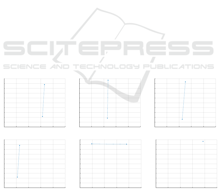
In Figure 4 we show the 6 resulting symbols in A

∗

Let us recall from Section 4.1 that the Letter datasets

have unlabelled edges and the nodes are labelled with

a 2D vector of hx, yi coordinates. For the sake of vi-

sualization, all hx,yi coordinates are scaled in the uni-

tary hypercube.

Certainly the most unexpected subgraph is de-

picted in Figure 4f: a single node in the top-right por-

tion of the hx,yi plane. Despite it appears trivial, an

end-point in the top-right portion is a feature which

is common in several capital Roman letters: amongst

the 15 letters (classes) it worth mentioning E, F, H,

K, M, N, T and Z.

Figure 4e shows another typical portion of many

capital Roman letters: a horizontal top line. This fea-

ture is less common with respect to the single node

(Figure 4f), yet it is characteristic of letters such as E,

F, T and Z.

Figures 4a–4d show a series of vertical or slightly

oblique lines, where the striking difference is in their

position along the x-axis. Many different capital Ro-

man letters can be drawn as a combination of these

‘basic’ traits: M, for example, is a combination of

4 vertical or slightly oblique lines (left to right: verti-

cal, oblique, oblique, vertical) and the same reasoning

holds for letters such as N, V, X and W.

However, it should be noted that the claim of

this a-posteriori validation is not that every letter

can be drawn by assembling the six symbols as de-

picted in Figure 4 as-they-are. In fact, we recall that

the similarity between graphs follows an inexact ap-

proach: this means that these symbols are likely to be

stretched or somehow moved across the hx,yi plane to

faithfully ‘match’ the drawing of capital Roman let-

ters (recall that the dissimilarity between nodes fol-

lows the Euclidean distance between their coordi-

nates). If the ‘as-they-are conjecture’ was true, then it

would have been impossible to recognize letters such

as E (which is one of the 15 letters to be classiﬁed)

0 0.2 0.4 0.6 0.8 1

0.1

0.2

0.3

0.4

0.5

0.6

0.7

0.8

0.9

(a)

0 0.2 0.4 0.6 0.8 1

0.1

0.2

0.3

0.4

0.5

0.6

0.7

0.8

0.9

(b)

0 0.2 0.4 0.6 0.8 1

0.1

0.2

0.3

0.4

0.5

0.6

0.7

0.8

0.9

(c)

0 0.2 0.4 0.6 0.8 1

0.1

0.2

0.3

0.4

0.5

0.6

0.7

0.8

0.9

(d)

0 0.2 0.4 0.6 0.8 1

0.1

0.2

0.3

0.4

0.5

0.6

0.7

0.8

0.9

(e)

0 0.2 0.4 0.6 0.8 1

0.1

0.2

0.3

0.4

0.5

0.6

0.7

0.8

0.9

(f)

Figure 4: Resulting symbols for Letter-L (10% subsampling rate, Mean operator).

NCTA 2021 - 13th International Conference on Neural Computation Theory and Applications

234

due to the absence of vertical lines positioned in the

middle and the bottom of the hx,yi-plane in the set of

symbols. However, there is an horizontal line (Fig-

ure 4e) that can easily be used to represent the three

horizontal lines in the letter E, counting three distinct

matches with different similarity degrees.

Relaxed Dissimilarity-based Symbolic Histogram Variants for Granular Graph Embedding

235