Allan Variance-based Granulation Technique for Large Temporal

Databases

Lorina Sinanaj

1 a

, Hossein Haeri

2 b

, Liming Gao

3 c

, Satya Prasad Maddipatla

3 d

Cindy Chen

1 e

, Kshitij Jerath

2 f

, Craig Beal

4 g

and Sean Brennan

3 h

Computer Science Department, University of Massachusetts Lowell, 220 Pawtucket St., Lowell, U.S.A.

Mechanical Engineering Department, University of Massachusetts Lowell, Lowell, U.S.A.

Mechanical Engineering Department, The Pennsylvania State University, University Park, U.S.A.

Mechanical Engineering Department, Bucknell University, Lewisburg, U.S.A.

Keywords:

Big Data, Data Reduction, Temporal Granulation, Allan Variance.

Abstract:

In the era of Big Data, conducting complex data analysis tasks efﬁciently, becomes increasingly important

and challenging due to large amounts of data available. In order to decrease query response time with limited

main memory and storage space, data reduction techniques that preserve data quality are needed. Existing

data reduction techniques, however, are often computationally expensive and rely on heuristics for deciding

how to split or reduce the original dataset. In this paper, we propose an effective granular data reduction tech-

nique for temporal databases, based on Allan Variance (AVAR). AVAR is used to systematically determine the

temporal window length over which data remains relevant. The entire dataset to be reduced is then separated

into granules with size equal to the AVAR-determined window length. Data reduction is achieved by gen-

erating aggregated information for each such granule. The proposed method is tested using a large database

that contains temporal information for vehicular data. Then comparison experiments are conducted and the

outstanding runtime performance is illustrated by comparing with three clustering-based data reduction meth-

ods. The performance results demonstrate that the proposed Allan Variance-based technique can efﬁciently

generate reduced representation of the original data without losing data quality, while signiﬁcantly reducing

computation time.

1 INTRODUCTION

Whether we are monitoring software systems, track-

ing applications, ﬁnancial trading analytics, business

intelligence tools, etc., time-series data ﬂows through

our data pipelines and applications at warp speed, en-

abling us to discover hidden and valuable information

on how that data changes over time. This has led to

a growing interest in the development of data mining

techniques capable in the automatic extraction of pat-

https://orcid.org/0000-0003-4687-5809

https://orcid.org/0000-0002-6772-6266

https://orcid.org/0000-0002-0159-4010

https://orcid.org/0000-0002-5785-3579

https://orcid.org/0000-0002-8712-8108

https://orcid.org/0000-0001-6356-9438

https://orcid.org/0000-0001-7193-9347

https://orcid.org/0000-0001-9844-6948

terns, anomalies, trends and other useful knowledge

from data (Johnston, 2001), (Liu and Motoda, 2002).

However, such hundreds of terabytes of data pose

an I/O bottleneck—both while writing the data into

the storage system and while reading the data back

during analysis. Given this magnitude and faced with

the curse of dimensionality which requires exponen-

tial running time to uncover signiﬁcant knowledge

patterns (Keogh and Mueen, 2017), much research

has been devoted to the data reduction task (Januzaj

et al., 2004). To make it beneﬁcial for data analysis,

it would be more convenient to deal with a reduced

set of representative and relevant dataset compared to

working on enormous amounts of raw and potentially

redundant data.

Traditional data reduction approaches have pro-

posed methods such as data compression (Rehman

et al., 2016), data cube aggregation (Gray et al.,

1997), sampling (Madigan and Nason, 2002), clus-

Sinanaj, L., Haeri, H., Gao, L., Maddipatla, S., Chen, C., Jerath, K., Beal, C. and Brennan, S.

Allan Variance-based Granulation Technique for Large Temporal Databases.

DOI: 10.5220/0010651500003064

In Proceedings of the 13th International Joint Conference on Knowledge Discovery, Knowledge Engineering and Knowledge Management (IC3K 2021) - Volume 3: KMIS, pages 17-28

ISBN: 978-989-758-533-3; ISSN: 2184-3228

tering (Kile and Uhlen, 2012), etc. The most notable

technique to reduce data with limited loss of impor-

tant information is to use cluster representatives in-

stead of the original instances. Unfortunately, widely-

used clustering methods such as K-means (MacQueen

et al., 1967), K-medoids (Kaufmann, 1987), Fuzzy

C-means (Bezdek et al., 1984), etc., can be compu-

tationally expensive and often rely on heuristics for

choosing the appropriate number of clusters to use.

To overcome these drawbacks, we propose a gran-

ularity reduction method based on Allan Variance

(AVAR) (Allan, 1966), (Haeri et al., 2021) for large

temporal databases. In this particular work we fo-

cus on the time-series data, where order and time are

fundamental elements that are crucial to the meaning

of the data, such that to predict what will happen at

a future time, information about the time when past

events occurred is needed. This is different from a

data stream analysis where time may not be an impor-

tant feature of the data. Such data streams can have

time-series data or non time-series data. The time

complexity of the proposed method is O(n) where n

is the number of input data points. This method uses

the concept of the time window over which measure-

ments are relevant, to systematically decide the size

of a data granule. After segmenting the time-series

dataset into granules according to the characteristic

timescale given by AVAR, we use the average value of

the granules as partition representatives instead of the

original data points. As a result, a reduced representa-

tion of the data is produced without losing important

information, while being computationally efﬁcient.

The rest of the paper is organized as follows. In

Section 2, we discuss related work. Section 3 de-

scribes the AVAR approach for ﬁnding the character-

istic timescale over which measurements are relevant.

The proposed algorithms and theoretical analysis of

the algorithms are presented in Section 4. The exper-

iments and results are demonstrated in Section 5. The

conclusions and future work follow in Section 6.

2 RELATED WORK

Granular computing is an information processing

paradigm to represent and process data into chunks

or clusters of information called information granules

(Pedrycz, 2001). Information granules are a collec-

tion of entities grouped together by similarity, prox-

imity, indistinguishability and functionality (Zadeh,

1997). The process of forming information granules

is called granulation. In this section, we brieﬂy re-

view the related work which investigate data reduc-

tion based on granules or clusters.

Lumini and Nanni (Lumini and Nanni, 2006)

present a data reduction method based on cluster-

ing (CLUT). The CLUT approach adopts the fuzzy

C-means clustering algorithm to divide the original

dataset into granules, then use the centroid of each

granule as the representative instance to achieve the

reduced dataset. The authors use the Hartigan’s

greedy heuristic (Hartigan, 1975) to select the optimal

number of clusters. The time complexity for the fuzzy

C-means method (Bezdek et al., 1984) is O(n

) with

the increase in the size of the original data, as a num-

ber of successive iterations need to be completed with

the intention to converge on an optimal set of parti-

tions. In addition, requiring a priori speciﬁcation of

the number of clusters by the Hartigan’s method, adds

more computational complexity to the overall cost.

Olvera et al. (Olvera-L

opez et al., 2010) achieve

data reduction by using a Prototype Selection based

Clustering method (PSC). PSC ﬁrst divides the orig-

inal dataset into clusters using the C-means algo-

rithm, then checks each cluster if it is homogeneous,

such that all instances belong to the same class, or

not. For the ﬁnal reduced prototype set, PSC selects

the set of the mean prototypes from each homoge-

neous cluster and the border prototypes from each

non-homogeneous cluster.

Sun et al. (Sun et al., 2019) propose to achieve

fast data reduction using granulation based instances

importance labeling (FDR-GIIL). The approach uses

K-means to generate the granules and then labels the

importance of each instance in each granule using the

Hausdorff distance (Henrikson, 1999). Data reduc-

tion is achieved by eliminating those instances which

have the lowest importance labels, until a user-deﬁned

reduction ratio is reached. However, K-means al-

gorithm (MacQueen et al., 1967) is computationally

expensive with high volume datasets. Similar to the

fuzzy C-means algorithm, when the number of input

data points n increases, it is observed that the time

complexity becomes O(n

For Big Data, the previous related works are time

consuming because the used clustering algorithms of-

ten rely on heuristics such as Hartigan’s statistics, rule

of thumb, elbow method, cross-validation, etc. (Kod-

inariya and Makwana, 2013) to choose the appropri-

ate number of clusters or granules. Additionally, they

need to process many iterations in order to converge

to optimal cluster centers. This leads to a quadratic

time complexity which is very prohibitive for large

datasets. To the best of our knowledge, this paper is

the ﬁrst to present a granular data reduction method

for temporal databases using Allan Variance, which

does not rely on heuristics and successive iterations

to process data into information granules.

KMIS 2021 - 13th International Conference on Knowledge Management and Information Systems

3 ALLAN VARIANCE

Allan Variance (AVAR) was ﬁrst proposed to charac-

terize the time drift in atomic clocks (Allan, 1966),

but later it became a practical method for sensor noise

characterization (Jerath et al., 2018). In its original

context, AVAR is often used to determine whether

noise values are correlated in time, and if they are,

it helps identify the correlation timescale. Drawing

inspiration from the classical applications of AVAR,

the authors recently proposed a novel method which

utilizes AVAR to identify the characteristic timescale

of any given temporal data set with numerical en-

tries (Haeri et al., 2021). Assuming a given noisy

temporal data follows a certain unknown pattern, the

characteristic timescale determines the time horizon

over which measurements yield a near-optimal mov-

ing average estimate (Haeri et al., 2021). Speciﬁcally,

our method suggests to consider measurements that

are not older than the characteristic timescale and use

them for estimation tasks.

3.1 AVAR-informed Characteristic

Timescale

Allan variance of a given temporal data set y =

,...,y

} is mathematically deﬁned as the ex-

pected variance of two successive averaged groups of

measurements, i.e. data blocks, at a given timescale

m (Allan, 1966), (Jerath et al., 2018):

(m) =



( ¯y

− ¯y

k−m

)



(1)

where ¯y

is simple moving average of the measure-

ments at time k and window length m, and is given

by:

¯y

∑

i=k−m

(2)

To numerically estimate AVAR, we can compute

average of the term ( ¯y

− ¯y

k−m

)

across all possible

time steps k (Sesia and Tavella, 2008):

(m) =

2(n − 2m)

∑

k=2m+1

( ¯y

− ¯y

k−m

)

(3)

A lower value of the AVAR at a given timescale

indicates lower bias and reduced variance between

data aggregated at that timescale. Depending on the

data patterns and noise characteristics, the variance

can increase or decrease as we increase the window

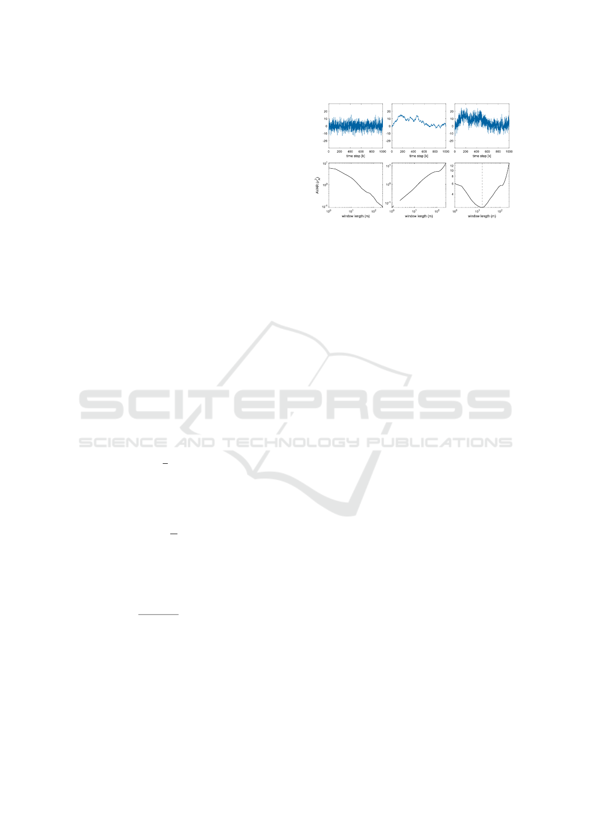
length or block size. Figure 1 shows three tempo-

ral signals and their corresponding AVAR calculated

Characteristic Timescale

x[k]

Noise (Uncorrelated) Signal (Correlated) Signal + Noise

(a) (b) (c)

(d) (e) (f)

Figure 1: Characteristic timescale determines the time hori-

zon over which averaging data points yields a near optimal

results. (a) Gaussian white noise (b) Random walk signal.

ure (d), (e), and (f) show AVAR of the signals on top calcu-

lated at various window lengths (1 ≤ m ≤ n/4).

at various timescales/window-lengths. Figure 1(d)

shows the AVAR for uncorrelated temporal data (in

this case Gaussian white noise). It is observed that

the AVAR decreases as the timescale or averaging

window lengths m increase. This is intuitive because

the aggregated data block values, i.e. ¯y

, approach

the mean value as the block size increases and more

samples are included in the average. On the other

hand, if data points are correlated in time, there is a

possibility of the Allan variance increasing with in-

creasing window lengths. For example, Figure 1(b)

shows a random walk process, and it is intuitively un-

derstood that the aggregates at varying timescales or

window lengths will drift apart over time, irrespec-

tive of the size of the aggregation timescale. Thus,

as seen in Figure 1(e), the AVAR increases as block

size increases since the data is correlated in time and

the most relevant measurements to any point at k is

its immediate neighboring measurement at k − 1 and

k + 1.

In this work, however, we are more interested in

cases like the one in Figure 1(c) where a correlated

signal is corrupted with an uncorrelated noise. In

this case, we are facing a trade-off where integrating

more data points help us eliminate the noise by per-

forming a moving averaging across a larger window

size but, at the same time, it would lower the accu-

racy by integrating less relevant measurements. The

proposed method suggests to choose a characteristic

timescale, i.e. the temporal aggregation timescale that

minimizes the AVAR.

3.2 Fast AVAR Calculation

Although AVAR yields valuable information regard-

ing the characteristic timescale of the temporal data,

it still needs to be efﬁciently computed for large data

Allan Variance-based Granulation Technique for Large Temporal Databases

sets. To accomplish this, we use the algorithm sug-

gested in (Prasad Maddipatla et al., 2021) and con-

strain the potential window lengths to powers of 2,

i.e m = 2

where p ∈ Z

. Then we can quickly es-

timate the expression in (1) using a simple dynamic

programming method with O(n) running time ex-

plained in Algorithm 1, where n is the number of

input data points. The algorithm ﬁrst constructs a

list of exponentially growing window length candi-

dates T . Then, for each window length, starting from

τ = 1, it calculates the associated AVAR by averaging

0.5(Y

−Y

k+1

)

across all valid k values. Meanwhile,

it pre-computes the next temporal list Y

by averaging

adjacent data values Y

and Y

k+1

Algorithm 1: Fast AVAR calculator.

Input: a set Y of raw temporal data points

Output: a set A of AVAR values and a set T

of associated timescales

construct T = {1,2,4,8,...,2

} such that

< Y.length/2 < 2

p+1

for τ ∈ T do

= empty list

k = 1

c = 0

while k < Y.length do

c = c + 0.5(Y

−Y

k+1

)

add 0.5(Y

k+1

) to Y

k = k + 2

end

add

.length

to A

Y = Y

end

return A and T

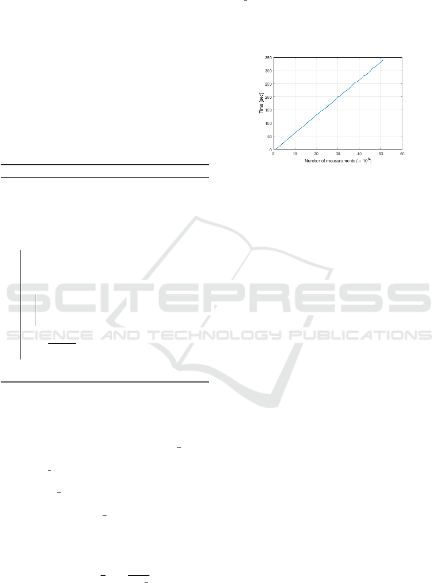
The theoretical analysis and the experiments in

Figure 2 prove that the running time for the Algorithm

1 is O(n). In the ﬁrst iteration where τ = 1, there will

be n × 1 calculations, in the second iteration because

τ = 2, the number of calculations will be n ×

, in the

third iteration τ = 4, so the number of AVAR calcula-

tions is n ×

and so on until the m-th iteration where

τ = 2

. In the last iteration the total number of calcu-

lations is n×(

)

. Adding all the calculations in each

iteration yields a geometric series with the ﬁrst term

is n, the common ratio is

, and the number of terms

is m. Using the sum formula for a ﬁnite geometric

series we can calculate the total time complexity of

Algorithm 1:

S =

∞

∑

p=0

)

1 −

(4)

Since the common ratio in this geometric series

(less than 1), the series converges with sum

S = O(n) = 2n. The linear complexity time of the fast

AVAR calculator is also shown in Figure 2, where the

execution time is linear and proportional to the num-

ber of measurements in the data.

Figure 2: Fast AVAR calculator execution time.

Being able to efﬁciently compute the AVAR char-

acteristic window length for large amounts of data

is crucial, because the number of the ﬁnal granules

or clusters in the reduced dataset is determined by

the temporal aggregation timescale given by the fast

AVAR algorithm.

4 AVAR-based GRANULATION

This section presents the structure of the pro-

posed AVAR-based granulation approach for tempo-

ral databases by describing the overall workﬂow of

the technique and the theoretical analysis of the algo-

rithm complexity, using the AVAR-informed charac-

teristic timescale.

4.1 System Architecture

The current state-of-the-art granulating temporal data

algorithms require successive iterations to be per-

formed as well as they rely on heuristics for choosing

how to partition the original data. This is a compu-

tationally expensive operation, especially for tempo-

ral databases with a large number of rows. The main

problem with using heuristics to specify the number

of clusters in advance, is that the ﬁnal result will be

sensitive to the initialization of parameters. A practi-

cal approach is to compare the outcomes of multiple

runs with different k-number of clusters and choose

the best one based on a predeﬁned criterion. How-

ever, this method is very time consuming due to the

large number of iterations that the algorithm needs to

carry out (MacQueen et al., 1967).

In our study, we propose an AVAR-based granu-

lation technique on large temporal databases, that in

KMIS 2021 - 13th International Conference on Knowledge Management and Information Systems

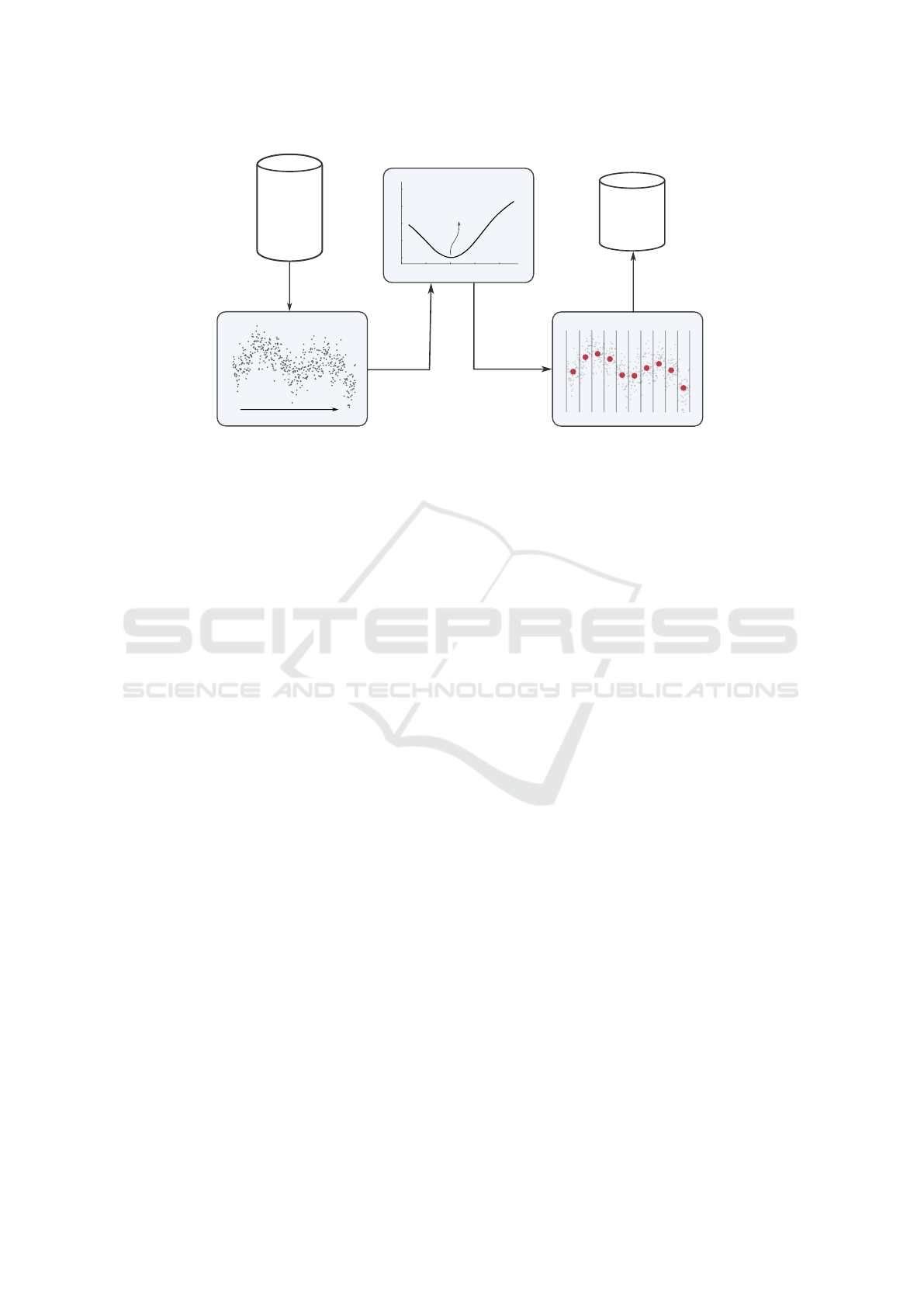
Characteristic Timescale

(block size)

AVAR

Time

Raw

Temporal

Database

Sort in time

Apply AVAR

Calculate

block averages

Insert

aggregated data

Reduced

Temporal

Database

Figure 3: System Architecture—Schematic view of data granulation process based on Allan Variance.

O(n) time complexity takes in input the n-raw data

points, systematically determines the time window

over which data is relevant, and calculates the aggre-

gated information of the relevant data for each time

window. Compared to previous approaches where

authors used heuristics (Kodinariya and Makwana,

2013) to determine the optimal number of partitions

(granules), in our work the number of partitions is

systematically determined by the AVAR characteris-

tic timescale.

Figure 3 shows the overall workﬂow of the

proposed method including four steps: (1) Pre-

processing: A simple pre-processing step is applied

on the raw dataset (if it is not originally sorted) to sort

the data points in time prior to applying the AVAR al-

gorithm, (2) Allan variance calculation: The AVAR

algorithm takes as input the sorted temporal database,

and outputs a characteristic timescale over which the

measurements are relevant and should be averaged

across, (3) Granulation: The granulation algorithm

takes in input the AVAR timescale, partitions the data

in a series of non-overlapping time interval segments

and generates aggregated information for each inter-

val, and (4) Data preparation: Aggregated informa-

tion for each partition will then be used as representa-

tive instances for the new reduced dataset. As a result,

at a later stage, data mining methods can analyze the

data faster due to the decrease in volume without los-

ing data quality.

Compared to the other methods in the related

works section, the AVAR-based technique systemat-

ically identiﬁes a characteristic timescale at which

measurements are relevant, representative and sta-

ble without relying on iterations or heuristics. As

a limitation to this method, input data should be

sorted in time before getting processed. However,

the worst-case time complexity when sorting the data

is O(nlog(n)) (Mishra and Garg, 2008), which still

has more advantage compared to methods that com-

pute a large number of iterations and use heuristics to

achieve approximate cluster representatives in O(n

4.2 AVAR Granulation Approach

A challenge in large sized databases is to evaluate

complex queries over a continuous stream of inputs.

The key idea is to reduce the volume using moving

window aggregations, i.e. the calculations of aggre-

gates in a series of non-overlapping (tumbling) win-

dows. Tumbling windows (Helsen et al., 2017) are

a series of ﬁxed-sized, non-overlapping, and contigu-

ous time intervals where tuples are grouped in a single

window based on time. A tuple in the database cannot

belong to more than one tumbling window. In the pro-

posed algorithm, AVAR method determines the size

of the tumbling window over which the measurements

are relevant.

The complete temporal granulation process de-

ﬁned according to the proposed methodology is de-

scribed by Algorithm 2. The algorithm takes as an

input the set of the original data points and the AVAR

characteristic timescale τ

AVAR

, and returns the set of

the granule representatives. Initially, it starts by se-

quentially scanning every data point in the original

set associated with their respective timestamp values.

It then partitions the data points into different time in-

tervals, by checking which window interval the times-

tamps fall into (if statement). Before jumping to a

new time window interval (else statement), the al-

gorithm calculates the average value for the current

granule and inserts that value in the representatives

set.

Allan Variance-based Granulation Technique for Large Temporal Databases

In Algorithm 2, the data is scanned only once in-

side the while loop. Each step inside the “if” and

“else” statements takes only O(1) time as it does

not contain loops, recursion or call to any other non-

constant time function. As a result, time complexity

of the AVAR-based granulation algorithm becomes

O(n), where n is the number of input data points. This

time complexity is linear and proportional to the size

of the original data. If we combine the time complex-

ity of Algorithm 1 with the time complexity of Al-

gorithm 2, the total time complexity of the proposed

approach is simply O(n). The more voluminous the

original data is, the slower the reduction algorithm

will be. However, our approach is a pre-processing

step to prepare the data for the future data analysing

techniques. Efﬁciency is achieved because data ana-

lytical methods can analyze the data faster due to the

decrease in volume without losing data quality.

The space complexity of the proposed algorithm

is the amount of memory space it needs to run ac-

cording to its input size. If the number of Information

Granules generated by the algorithm is q and the input

size is n, the storage requirement for the algorithm to

complete its task is O(nq).

Algorithm 2: AVAR-based temporal granulation al-

gorithm.

Input: a set Y of raw temporal data points

and timescale τ

AVAR

Output: a set Y ’ of granule representatives

initialize window

start

and window

size

=τ

AVAR

q=1 // Information Granules counter

while y ∈ Y do

if timestamp(y) ∈ window interval then

insert y in Information Granule IG

else

set window

start

(window

start

+window

size

)

shift window interval (window

start

window

start

+window

size

)

calculate the average ¯y

for all

y ∈ IG

add ¯y

to Y ’

q=q+1

end

return Y ’

5 EXPERIMENTS

In the following we present experimental results that

assess the performance of the AVAR method in the

granulation algorithm. As the experimental basis, a

simulation environment is used to produce a large

amount of temporal information for vehicular data.

Each tuple contains information about road-tire fric-

tion measurements at a certain point in time.

On this dataset we perform three separate experi-

ments: (1) we apply the AVAR method to determine

the characteristic timescale over which measurements

are relevant, (2) we apply the granulation algorithm

based on the AVAR output, on data of different sizes

to observe the algorithm execution time with respect

to input data size, and (3) on the input dataset and on

the reduced dataset, we run the same exact query to

analyze the performance of our reduction method. In

addition experimental analysis is conducted to com-

pare the proposed method against the competitors in

the related works.

The test results show that performing the same

type of query in the reduced dataset compared to ex-

ecuting the query in the original data, not only drasti-

cally reduces the query execution time but it can also

generate close results with a relatively low absolute

error.

Hardware: The platform of our experimentation is a

PC with a 2.60 GHz Single Core CPU, 64 GB RAM

using PostgreSQL 10.12 on Linux kernel 3.10.0.

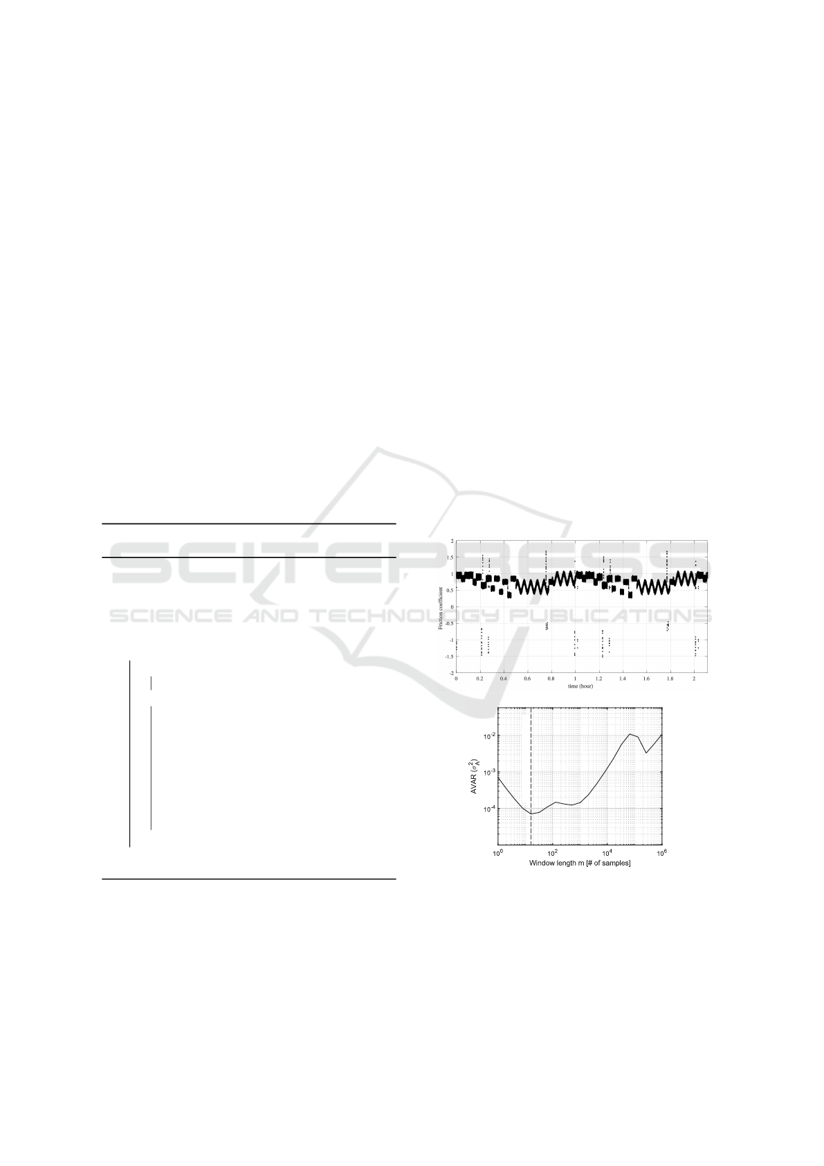
Characteristic timescale (m=16)

Figure 4: Top: Friction data. Negative values are outliers

but we retained them to show that the technique is robust

under different scenarios. Bottom: Allan variance for ve-

hicular friction measurements containing 91 million data

points, evaluated across various window lengths.The min-

imum point in the AVAR curve indicates the characteristic

timescale of the data.

KMIS 2021 - 13th International Conference on Knowledge Management and Information Systems

5.1 Characteristic Timescale of

Vehicular Data

In this subsection, we evaluate the characteristic

timescale of the vehicular friction measurements by

calculating the AVAR across various window lengths

using the Algorithm 1. Figure 4(Top) shows the

pattern of the friction values over time and Figure

4(Bottom) shows the corresponding AVAR curve.

5.2 Time Efﬁciency of AVAR-based

Granulation Algorithm

To measure the time efﬁciency of the AVAR-based

granulation algorithm, we will gradually increment

the size of the data to be granulated. We initially start

by applying the granulation algorithm on a temporal

database of size 2.5 GB (≈ 32 million data points),

and we measure its execution time. We repeat these

steps by applying the algorithm on data with differ-

ent sizes up to 25 GB (≈ 320 million data points) and

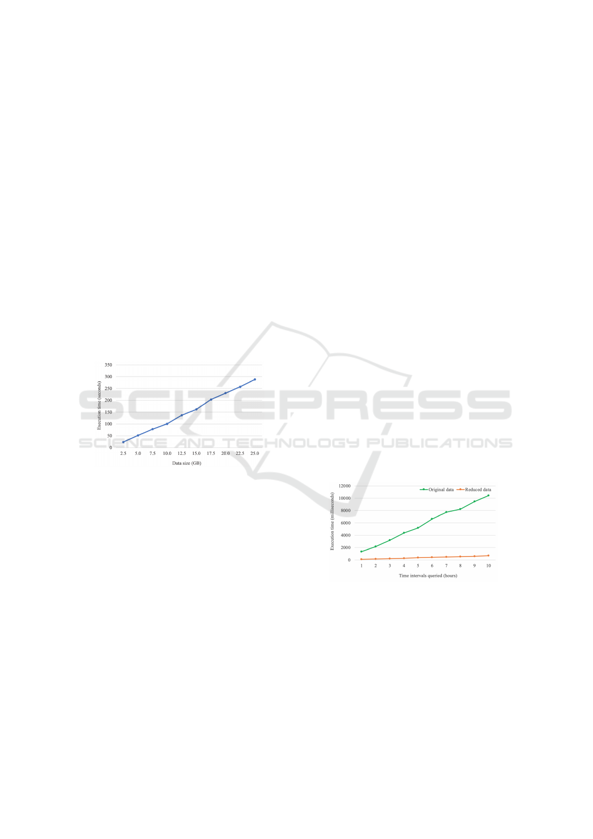
present the results in Figure 5.

Figure 5: Execution time of the AVAR-based granulation

algorithm.

From these results, we observe that for larger

amounts of input data, the algorithm takes more time

to execute. However, the increase in execution time is

linear to the size of the input data, once again prov-

ing our theoretical algorithm analysis that the time

complexity for our proposed AVAR-based granulation

technique is O(n), where n is the number of input data

points.

5.3 Effectiveness of AVAR-based

Granulation Technique

We evaluate the proposed approach on a vehicular in-

formation dataset of size 7216 MB, which consists of

91,475,050 tuples measured at a time range of around

25 hours. Each tuple holds road-tire friction val-

ues associated with their respective timestamps. The

purpose of AVAR-based granulation is to reduce the

query execution time without losing important infor-

mation from data reduction. To show that this tech-

nique efﬁciently produces a reduced representation of

the data without losing data quality, we run the same

query on both datasets, the original and the reduced,

and we analyze the query execution time as well as

the query results. We use a query to output the av-

erage friction value for a given interval in time. The

query is run for different time intervals, to observe

how the query execution time changes when an in-

creasingly number of tuples have to be analyzed. We

show that after using our approach, data can be an-

alyzed faster due to the decrease in volume, without

losing important information.

First, we show that the query execution time can

be reduced drastically after applying the AVAR-based

granulation algorithm. The size of the reduced dataset

after the granulation technique with a characteristic

timescale of 16 milliseconds is 426 MB, with the

total number of tuples being 5,717,191. The storage

requirement is efﬁciently reduced as shown by the

calculated reduction rate of ≈ 94 %. Experimental

results in Figure 6 show that for the same time

interval, the query takes less time to execute in the

reduced data compare to executing it in the original

data. In addition, we observe that for the original

dataset, the runtime growth of the query is higher

with the growth of the amount of data queried. From

these results we can observe that the beneﬁts of data

reduction processes are sometimes not evident when

the data is small; they begin to become obvious when

the datasets start growing in size and more instances

have to be analyzed.

Figure 6: The runtime rising tendency of the query as more

data is analyzed

Second, we show that we do not lose data quality

while reducing the temporal database in a representa-

tive subset. The advantage of using representatives is

that besides improving query execution time, it also

improves the model generalization for the use of data

mining techniques in the future. We measured the

average, minimum and maximum friction values for

different time intervals on both datasets. Numerical

results are shown in Table 1.

Allan Variance-based Granulation Technique for Large Temporal Databases

Table 1: Query performance on the friction data.

AVG(friction) AVG query error MIN(friction) MIN query error MAX(friction) MAX query error

Interval of time

Original data Reduced data Percentage Absolute Original data Reduced data Percentage Absolute Original data Reduced data Percentage Absolute

between ’2020-06-15

05:00:00’ and ’2020-06-15

05:10:00’

0.754902 0.754902 1.14E-05 8.60E-08 -1.608 -0.929 42.214 0.679 1.559 1.326 14.968 0.233

between ’2020-06-15

05:10:00’ and ’2020-06-15

05:20:00’

0.654777 0.654776 1.05E-04 6.87E-07 0.253 0.324 28.170 0.071 0.949 0.870 8.349 0.079

between ’2020-06-15

05:20:00’ and ’2020-06-15

05:30:00’

0.600036 0.600037 1.97E-04 1.18E-06 0.349 0.431 23.460 0.082 0.839 0.770 8.246 0.069

between ’2020-06-15

05:30:00’ and ’2020-06-15

05:40:00’

0.686079 0.686078 1.46E-04 1.00E-06 -0.723 -0.258 64.385 0.466 1.732 1.532 11.571 0.200

between ’2020-06-15

05:40:00’ and ’2020-06-15

05:50:00’

0.849033 0.849026 8.27E-04 7.02E-06 -1.536 -1.011 34.193 0.525 1.413 1.084 23.317 0.329

between ’2020-06-15

05:50:00’ and ’2020-06-15

06:00:00’

0.897936 0.897934 2.36E-04 2.12E-06 0.633 0.728 14.931 0.095 1.074 0.975 9.214 0.099

From Table 1 we can observe that for the aver-

age (AVG) query, the error is occurring at the 5

decimal place. This event mostly happens due

to the computer representation for binary ﬂoating-

point numbers in the IEEE Standard for Floating-

Point Arithmetic (IEEE 754)(IEEE, 2019). IEEE

754 standard, for ﬂoating point representation, al-

lows 23 bits for the fraction. 23 bits is equivalent

to log

(23) ≈ 6 decimal digits. Beyond those num-

ber of signiﬁcant digits, accuracy is not preserved,

hence round-off starts to occur as reported in Table

1. The absolute error values, mostly due to numeri-

cal accuracy round-off, are extremely small, proving

that the AVAR-based granulation technique in tempo-

ral databases keeps the quality of the original data.

Nevertheless, the vehicular friction values round to

the 4

decimal place, already have enough accuracy

for vehicular control application.

For the minimum (MIN) and maximum (MAX)

queries, even though the absolute error is larger due

to the presence of outliers (as observed in Figure

4(Top)), the results are still close in value to each

other. A good approach in the future is to apply a

ﬁltering algorithm that removes the outliers prior to

applying the AVAR granulation approach.

5.4 Comparative Evaluation

Comparison experiments are conducted by compar-

ing the proposed AVAR-based granulation algorithm

with the other clustering data reduction methods in

the related works. Five datasets selected from the UCI

Repository (Dua and Graff, 2019) with different sizes

are reduced to demonstrate the effectiveness of the

AVAR approach. The chosen datasets (Segmentation,

Magic, Letter, Shuttle, Covertype) are considered as

“large” datasets by the competitors FDR-GIIL (Sun

et al., 2019), CLU (Lumini and Nanni, 2006) and PSC

(Olvera-L

opez et al., 2010). CLU and PSC are not ap-

plicable to run in the Covertype dataset (250,000 in-

stances), because they are very expensive when large

datasets are processed. A description of these datasets

is given in Table 2.

Table 2: Description of datasets.

Dataset

Number of

instances

Number of

attributes

Segmentation 2100 19

Magic 19,020 10

Letter 20,000 16

Shuttle 58,000 9

Covertype 250,000 54

There are two key experiments conducted in this

section; (i) measurement of the query performance

in each dataset after they have been reduced by the

AVAR-based approach and (ii) evaluation of how fast

the execution time of the proposed AVAR approach is

compared to the existing clustering based data reduc-

tion methods.

Figure 7, 8, 9, 10 and 11 show the AVAR calcu-

lated at various window lengths for each dataset. We

can observe from the graphs in Figures 7-11(a), how

each data has different characteristics and shapes.

Some of them have a large number of outliers (Shuttle

and Covertype), while some others have many repet-

itive data points (Letter). It is important to see how

the AVAR-method performs against different kind of

data, so that future work can be planned to make the

method applicable in more general cases.

The ﬁrst step in the proposed granulation process

measures the characteristic window length at the min-

imum AVAR, shown in Figures 7-11(b). The next step

is to use this window length to separate the data into

granules and generate the aggregated information for

each such granule. After the reduction step is per-

formed, we observe the query performance for each

reduced dataset.

KMIS 2021 - 13th International Conference on Knowledge Management and Information Systems

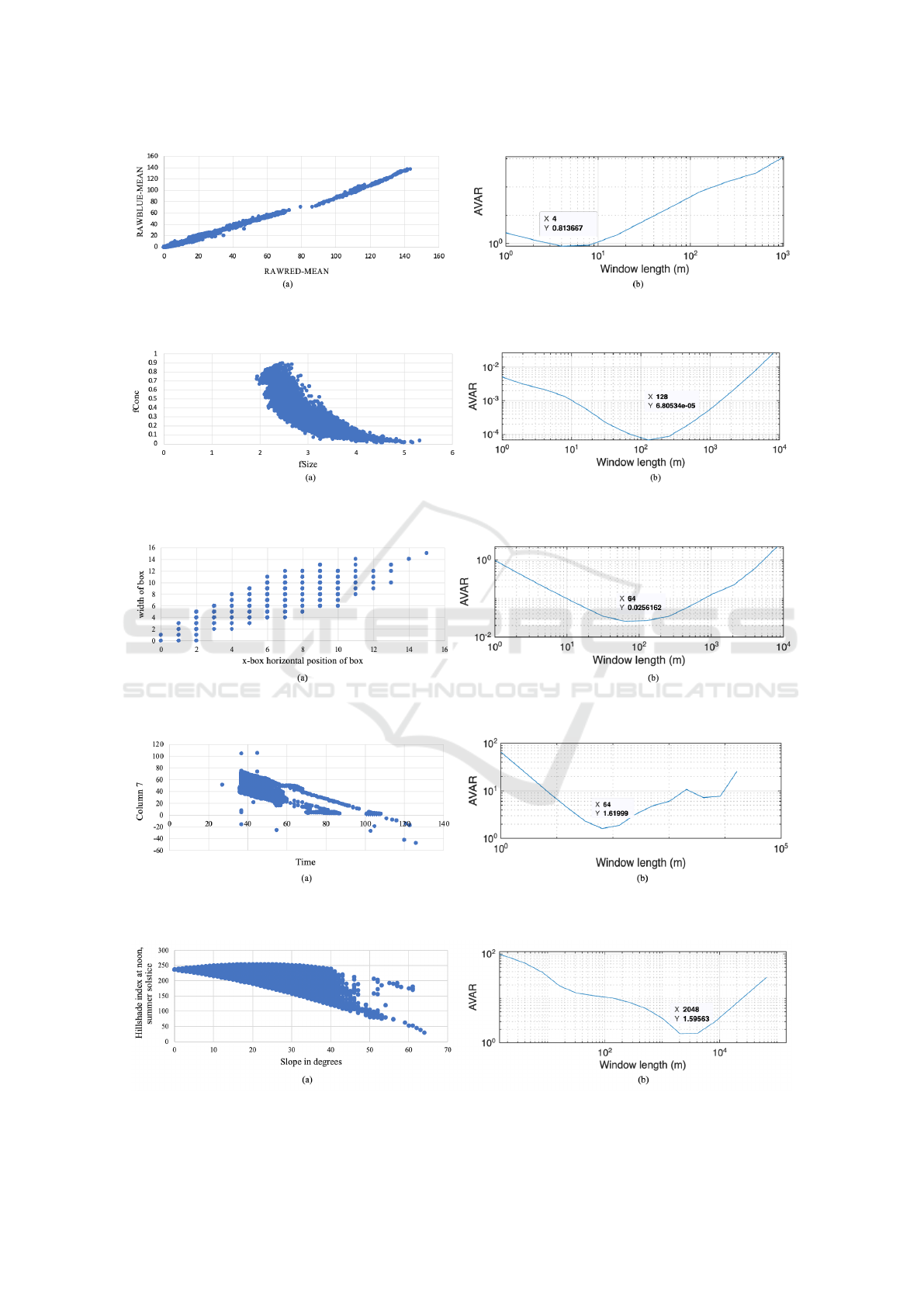
Figure 7: AVAR of the Segmentation dataset calculated at various window lengths. (a)Segmentation data (b)AVAR curve

showing the characteristic window length=4 units.

Figure 8: AVAR of the Magic dataset calculated at various window lengths. (a) Magic data (b) AVAR curve showing the

characteristic window length = 128 units.

Figure 9: AVAR of the Letter dataset calculated at various window lengths. (a) Letter data (b) AVAR curve showing the

characteristic window length = 64 units.

Figure 10: AVAR of the Shuttle dataset calculated at various window lengths. (a) Shuttle data (b) AVAR curve showing the

characteristic window length = 64 units.

Figure 11: AVAR of the Covertype dataset calculated at various window lengths. (a) Covertype data (b) AVAR curve showing

the characteristic window length = 2048 units.

Allan Variance-based Granulation Technique for Large Temporal Databases

Table 3: Query performance on the Segmentation data.

AVG(RAWBLUE-MEAN) AVG query error MIN(RAWBLUE-MEAN) MIN query error MAX(RAWBLUE-MEAN) MAX query error

Interval of

RAWRED-MEAN

Original data Reduced data Percentage Absolute Original data Reduced data Percentage Absolute Original data Reduced data Percentage Absolute

[0, 29] 9.506 9.506 0.000 0.000 0.000 0.000 0.000 0.000 26.111 25.083 3.937 1.028

[29, 58] 39.698 39.778 0.202 0.080 18.333 24.417 33.186 6.084 54.111 51.639 4.568 2.472

[58, 87] 55.188 55.161 0.049 0.027 50.000 51.278 2.556 1.278 70.778 65.389 7.614 5.389

[87, 116] 92.963 92.877 0.093 0.086 72.000 72.250 0.347 0.250 107.444 103.639 3.541 3.805

[116, 145] 118.453 118.543 0.076 0.090 103.667 105.778 2.036 2.111 137.111 136.000 0.810 1.111

Table 4: Query performance on the Magic data.

AVG(fConc) AVG query error MIN(fConc) MIN query error MAX(fConc) MAX query error

Interval of fSize

Original data Reduced data Percentage Absolute Original data Reduced data Percentage Absolute Original data Reduced data Percentage Absolute

[2.0, 2.5] 0.594 0.596 0.337 0.002 0.290 0.492 69.655 0.202 0.893 0.734 17.805 0.159

[2.5, 3.0] 0.377 0.378 0.265 0.001 0.116 0.265 128.448 0.149 0.885 0.49 44.633 0.395

[3.0, 3.5] 0.221 0.221 0.000 0.000 0.049 0.174 255.102 0.125 0.638 0.262 58.934 0.376

[3.5, 4.0] 0.153 0.154 0.654 0.001 0.025 0.120 380.000 0.095 0.292 0.177 39.384 0.115

[4.0, 4.5] 0.080 0.085 6.250 0.005 0.013 0.068 423.077 0.055 0.155 0.102 34.194 0.053

Table 5: Query performance on the Letter data.

AVG(box width) AVG query error MIN(box width) MIN query error MAX(box width) MAX query error

Interval of

horizontal position

Original data Reduced data Percentage Absolute Original data Reduced data Percentage Absolute Original data Reduced data Percentage Absolute

[0, 3] 2.592 2.610 0.694 0.018 0.000 0.281 0.000 0.281 5.000 3.906 21.880 1.094

[3, 6] 5.235 5.243 0.153 0.008 2.000 4.156 107.800 2.156 9.000 6.516 27.600 2.484

[6, 9] 7.408 7.409 0.013 0.001 4.000 6.703 67.575 2.703 12.000 8.297 30.858 3.703

[9, 12] 8.567 8.567 0.000 0.000 6.000 7.797 29.950 1.797 14.000 9.703 30.693 4.297

[12, 15] 11.259 11.375 1.030 0.116 9.000 11.375 26.389 2.375 14.000 11.375 18.750 2.625

Table 6: Query performance on the Shuttle data.

AVG(column 7) AVG query error MIN(column 7) MIN query error MAX(column 7) MAX query error

Interval of time

Original data Reduced data Percentage Absolute Original data Reduced data Percentage Absolute Original data Reduced data Percentage Absolute

[25, 45] 44.626 44.625 0.002 0.001 -16.000 37.531 334.569 53.531 104.000 50.750 51.202 53.250

[45, 65] 34.178 34.178 0.000 0.000 -26.000 28.000 207.692 54.000 105.000 48.016 54.270 56.984

[65, 85] 6.857 6.720 1.998 0.137 3.000 3.188 6.267 0.188 48.000 44.078 8.171 3.922

[85, 105] 2.156 2.039 5.427 0.117 -27.000 0.565 102.093 27.565 22.000 5.516 74.927 16.484

[105, 125] 0.321 -2.560 897.508 2.881 -43.000 -20.688 51.888 22.312 3.000 1.203 59.900 1.797

Table 7: Query performance on the Covertype data.

AVG(hillshade index noon) AVG query error MIN(hillshade index noon) MIN query error MAX(hillshade index noon) MAX query error

Interval of slope

Original data Reduced data Percentage Absolute Original data Reduced data Percentage Absolute Original data Reduced data Percentage Absolute

[0, 10] 232.452 232.383 0.030 0.069 219.000 227.854 4.043 8.854 249.000 237.337 4.684 11.663

[10, 20] 222.861 222.766 0.043 0.095 194.000 213.032 9.810 19.032 254.000 229.754 9.546 24.246

[20, 30] 204.780 204.199 0.284 0.581 162.000 190.453 17.564 28.453 254.000 212.414 16.372 41.586

[30, 40] 184.955 182.371 1.397 2.584 126.000 172.000 36.508 46.000 252.000 190.098 24.564 61.902

[40, 50] 149.370 122.424 18.040 26.946 87.000 122.424 40.717 35.424 240.000 122.424 48.990 117.576

For the Segmentation dataset, we measured the

average, minimum and maximum rawblue values

where rawred was between a given interval. For

the Magic dataset, we measured the average, mini-

mum and maximum fConc values where fSize was

between a given interval. For the Letter dataset,

we measured the average, minimum and maximum

box width values where horizontal position was

between a given interval. For the Shuttle dataset,

we measured the average, minimum and maxi-

mum Column 7 values where time was between

a given interval. For the Covertype dataset, we

measured the average, minimum and maximum

hillshade index noon values where slope was be-

tween a given interval.

KMIS 2021 - 13th International Conference on Knowledge Management and Information Systems

Table 8: Execution time of large datasets (seconds).

Execution time (seconds)

Dataset Number of instances Number of attributes

AVAR

window size

AVAR FDR-GIIL CLU PSC

Segmentation 2100 19 4 0.286 3.9 6.0 7.0

Magic 19,020 10 128 0.217 88.6 167.1 172.1

Letter 20,000 16 64 0.210 14.5 217.2 226.2

Shuttle 58,000 9 64 0.351 30.9 277.4 288.4

Covertype 250,000 54 2048 0.321 649.7 - -

Numerical results for each data are shown in Ta-

bles 3, 4, 5, 6 and 7. For the AVERAGE query we

can observe that the absolute error is almost always

close to 0, indicating that there is little difference be-

tween the results in the original and the reduced data.

There are special cases where the absolute error is

large, as in certain intervals of Table 6 and 7 which

is explained by the presence of outliers in those in-

tervals of the original data. The presence of outliers

has a more obvious effect in the results of the MINI-

MUM and MAXIMUM queries. In such queries there

is a larger gap in the results between the original and

the reduced data, hence the absolute error is worse.

As a recommendation in the future, a ﬁltering algo-

rithm for the outliers removal will be used before the

AVAR-based granulation approach. As the number of

outliers increases, so does the absolute error.

While the competitors pick K-means or fuzzy C-

means to decide on the number of clusters, the AVAR

approach sets the size of the cluster by using the char-

acteristic window length on available data. The com-

parative experiments show that the AVAR-method can

still give good performance results in preserving data

quality even in data streams that are not time-series.

In the future we plan to extend this approach for both

spatio-temporal data. Next, the execution time of the

competitor algorithms FDR-GIIL, CLU and PSC are

added for each dataset to show the improvement in

the computational cost of the proposed AVAR-based

granulation method. The corresponding results are

recorded in Table 8. The ‘-’ sign indicates that the ex-

ecution time of the algorithm is more than 100 hours,

as we can see for CLU and PSC which have an expen-

sive computational cost when data increases in size

(Covertype data). Nevertheless, we have shown that

the AVAR approach can be executed for data up to

≈ 90,000,000 instances (friction data). For temporal

data, while the other approaches perform two dimen-

sional clustering, the AVAR approach generates clus-

ters based on the characteristic timescale. The AVAR-

based method will offer fewer advantages for datasets

that are more complex or for which averaging is less

useful.

When the characteristic AVAR window size is

small, the number of the representative prototypes

is larger, hence there is a higher insertion cost of

these instances in the new reduced table (Segmenta-

tion dataset). When the characteristic AVAR window

size is large, the number of the representative proto-

types is smaller, hence there is a lower insertion cost

of these instances in the new reduced table (Magic

dataset). When the characteristic AVAR window size

is the same for two different datasets, the dataset with

a larger number of instances will have a higher com-

putational cost than the dataset with a lower number

of instances (Letter and Shuttle datasets). From Table

8 it can be concluded that the execution time of our

algorithm is much smaller than the compared algo-

rithms, proving once again that the AVAR approach is

fast when applied on Big data.

6 CONCLUSIONS AND FUTURE

WORK

In this paper we have proposed a computation-

ally efﬁcient granulation algorithm for large tempo-

ral databases using Allan Variance. The proposed

method systematically determines the characteristic

timescale over which data is relevant and calculates

the aggregated information for each time window.

The total time complexity of this approach is O(n),

which is an improvement from existing algorithms

O(n

). Experimental results show that the proposed

technique considerably reduces the query execution

time by reducing the storage requirement, while pre-

serving data integrity. Overall, the presented ap-

proach increases query efﬁciency due to the decrease

in data volume while preserving the quality of the re-

sult of the queries.

In the future, we plan to incorporate an outlier-

removal ﬁltering algorithm to our method and further

improve this approach for spatio-temporal databases

with respect to both their time domain and spatial

layouts. One interesting challenge is that in multi-

Allan Variance-based Granulation Technique for Large Temporal Databases

dimensional data, different granularities may exist.

Choosing the appropriate level of detail or granularity

is crucial. To mitigate this challenge, we plan to ex-

tend the AVAR-based approach to represent different

levels of resolution by creating a hierarchical struc-

ture of spatio-temporal data. In addition, we will fo-

cus whether and when to recalculate the characteristic

timescale, as the AVAR estimator would be useful in

an incremental scenario when data keeps coming in.

Furthermore, we intend to construct dynamic AVAR

estimators which can cope with local changes in the

temporal and spatial characteristic sizes.

REFERENCES

Allan, D. W. (1966). Statistics of atomic frequency stan-

dards. Proceedings of the IEEE, 54(2):221–230.

Bezdek, J. C., Ehrlich, R., and Full, W. (1984). FCM:

The fuzzy c-means clustering algorithm. Computers

& Geosciences, 10(2-3):191–203.

Dua, D. and Graff, C. (2019). UCI machine learning repos-

itory, 2017. URL http://archive.ics.uci.edu/ml.

Gray, J., Chaudhuri, S., Bosworth, A., Layman, A., Re-

ichart, D., Venkatrao, M., Pellow, F., and Pirahesh, H.

(1997). Data cube: A relational aggregation operator

generalizing group-by, cross-tab, and sub-totals. Data

Mining and Knowledge Discovery, 1(1):29–53.

Haeri, H., Beal, C. E., and Jerath, K. (2021). Near-

optimal moving average estimation at characteristic

timescales: An Allan variance approach. IEEE Con-

trol Systems Letters, 5(5):1531–1536.

Hartigan, J. A. (1975). Clustering algorithms. John Wiley

& Sons, Inc.

Helsen, J., Peeters, C., Doro, P., Ververs, E., and Jordaens,

P. J. (2017). Wind farm operation and maintenance

optimization using big data. In 2017 IEEE Third Inter-

national Conference on Big Data Computing Service

and Applications (BigDataService), pages 179–184.

Henrikson, J. (1999). Completeness and total boundedness

of the hausdorff metric. MIT Undergraduate Journal

of Mathematics, 1:69–80.

IEEE (2019). IEEE standard for ﬂoating-point arithmetic.

IEEE Std 754-2019 (Revision of IEEE 754-2008),

pages 1–84.

Januzaj, E., Kriegel, H.-P., and Pfeiﬂe, M. (2004). Dbdc:

Density based distributed clustering. In Interna-

tional Conference on Extending Database Technol-

ogy, pages 88–105. Springer.

Jerath, K., Brennan, S., and Lagoa, C. (2018). Bridging the

gap between sensor noise modeling and sensor char-

acterization. Measurement, 116:350 – 366.

Johnston, W. (2001). Model Visualization, page 223–227.

Morgan Kaufmann Publishers Inc., San Francisco,

CA, USA.

Kaufmann, L. (1987). Clustering by means of medoids. In

Proc. Statistical Data Analysis Based on the L1 Norm

Conference, Neuchatel, 1987, pages 405–416.

Keogh, E. and Mueen, A. (2017). Curse of dimensional-

ity. In Encyclopedia of Machine Learning and Data

Mining, pages 314–315.

Kile, H. and Uhlen, K. (2012). Data reduction via clustering

and averaging for contingency and reliability analysis.

International Journal of Electrical Power & Energy

Systems, 43(1):1435–1442.

Kodinariya, T. M. and Makwana, P. R. (2013). Review on

determining number of cluster in k-means clustering.

International Journal, 1(6):90–95.

Liu, H. and Motoda, H. (2002). On issues of instance selec-

tion. Data Min. Knowl. Discov., 6:115–130.

Lumini, A. and Nanni, L. (2006). A clustering method

for automatic biometric template selection. Pattern

Recognition, 39(3):495–497.

MacQueen, J. et al. (1967). Some methods for classiﬁcation

and analysis of multivariate observations. In Proceed-

ings of the Fifth Berkeley symposium on mathematical

statistics and probability, volume 1, pages 281–297.

Oakland, CA, USA.

Madigan, D. and Nason, M. (2002). Data reduction: sam-

pling. In Handbook of data mining and knowledge

discovery, pages 205–208.

Mishra, A. D. and Garg, D. (2008). Selection of best sorting

algorithm. International Journal of intelligent infor-

mation Processing, 2(2):363–368.

Olvera-L

opez, J. A., Carrasco-Ochoa, J. A., and Mart

ınez-

Trinidad, J. F. (2010). A new fast prototype selection

method based on clustering. Pattern Analysis and Ap-

plications, 13(2):131–141.

Pedrycz, W. (2001). Granular computing: an introduc-

tion. In Proceedings joint 9th IFSA world congress

and 20th NAFIPS international conference (Cat. No.

01TH8569), volume 3, pages 1349–1354. IEEE.

Prasad Maddipatla, S., Haeri, H., Jerath, K., and Bren-

nan, S. (To appear in October 2021). Fast Allan vari-

ance (FAVAR) and dynamic fast Allan variance (D-

FAVAR) algorithms for both regularly and irregularly

sampled data. Modeling, Estimation and Control Con-

ference.

Rehman, M. H., Liew, C. S., Abbas, A., Jayaraman, P. P.,

Wah, T. Y., and Khan, S. U. (2016). Big data reduction

methods: a survey. Data Science and Engineering,

1(4):265–284.

Sesia, I. and Tavella, P. (2008). Estimating the Allan vari-

ance in the presence of long periods of missing data

and outliers. Metrologia, 45(6):S134.

Sun, X., Liu, L., Geng, C., and Yang, S. (2019). Fast data re-

duction with granulation-based instances importance

labeling. IEEE Access, 7:33587–33597.

Zadeh, L. A. (1997). Toward a theory of fuzzy information

granulation and its centrality in human reasoning and

fuzzy logic. Fuzzy sets and systems, 90(2):111–127.

KMIS 2021 - 13th International Conference on Knowledge Management and Information Systems