Medoid-based MLP: An Application to Wood Sawing Simulator

Metamodeling

Sylvain Chabanet

, Philippe Thomas

and Hind Bril El-Haouzi

Universit

e de Lorraine, CNRS, CRAN, F-88000 Epinal, France

Keywords:

MLP, Regressor Ensemble, Sawmill Simulation, ICP Dissimilarity, Medoid.

Abstract:

Predicting the set of lumbers which would be obtained from sawing a log at a speciﬁc sawmill is a difﬁcult

problem, which complicates short and mid term decision making in this industry. While sawmill simulators

able to simulate the sawing of a log from a 3D scan of its outer shape exist, they can be extremely compu-

tationally intensive. Several alternative approaches based on machine learning algorithms and different set

of features were explored in previous works. This paper proposes the use of one hidden layer perceptrons,

and a vector of features build from dissimilarities from the scans to a set of selected wood logs, chosen as

the class medoids. Several architectures are tested and compared to validate the pertinence of the proposed

set of medoid-based features. The lowest mean squared error was obtained for MISO neural networks with a

sigmoid output activation function, to constrain the output value ranges.

1 INTRODUCTION

As is reﬂected by the scientiﬁc literature, artiﬁcial

intelligence tools, including neural networks, could

advantageously intervene at different levels of the

forest-wood industry. A popular application seems,

for example, to be the processing of remote sens-

ing data. For example, (Del Frate and Solimini,

2004) assesses the interest of Multi Layers Percep-

tron (MLP) models to evaluate forest biomass from

airborne laser data. Recently, (Zhang et al., 2020)

proposed a lightweight convolutional neural network

(CNN) architecture to classify tree species using air-

borne multi-spectral imagery. Similarly, (Sylvain

et al., 2019) uses an ensemble of deep CNN to map

dead trees from aerial photographs. An advantage of

using remote sensing technologies and artiﬁcial intel-

ligence algorithms in these cases is that they limit the

need for time consuming and labor intensive ground

studies in areas sometime difﬁcult to access on foot.

As example of other applications of neural networks

to the forest wood industry, (Thomas and Thomas,

2011) uses a MLP to reduce a sawmill workshop sim-

ulation model, focusing on bottlenecks. Addition-

ally, (Wenshu et al., 2015) studies the use of Artiﬁcial

Neural Networks to classify wood defects on boards.

https://orcid.org/0000-0002-3706-293X

https://orcid.org/0000-0001-9426-3570

https://orcid.org/0000-0003-4746-5342

Their ﬁnal objective is to improve sawmills lumber

recovery.

A particularity of the sawing process is that the

set of lumbers which can be obtained by processing

a speciﬁc log at a sawmill with a given conﬁguration,

called in this study a basket of products, can be difﬁ-

cult to predict in advance. This is due, in particular, to

the heterogeneity of the raw material. Each log has a

speciﬁc shape, quality, and defects, all of which inﬂu-

ence the ﬁnal set of products. In addition, the sawing

process itself is divergent with co-production. This

means that several lumbers, and other co-products,

are simultaneously sawed from the same log. Lum-

bers sawed from a same log, in particular, may have

various dimensions and grades. This introduces un-

certainty in the production process and complicates

decision making. For example, as explained in (Wery

et al., 2018), the acceptation by a sawmill of an or-

der with unusual products would require to change the

sawmill conﬁguration. This would impact the whole

lumber mix produced, in a way which is difﬁcult to

predict. Other studies, like (Morneau-Pereira et al.,

2014) propose a Mixed-Integer Programming (MIP)

model to optimize the allocation of wood logs from

cut blocks to sawmills. Such a MIP model requires,

however, at least an estimation of what can be ob-

tained from the set of logs at each sawmill. Both of

these authors use simulation tools to generate the data

needed for their respective models.

Chabanet, S., Thomas, P. and El-Haouzi, H.

Medoid-based MLP: An Application to Wood Sawing Simulator Metamodeling.

DOI: 10.5220/0010651400003063

In Proceedings of the 13th International Joint Conference on Computational Intelligence (IJCCI 2021), pages 201-210

ISBN: 978-989-758-534-0; ISSN: 2184-3236

201

Figure 1: Sawing is a divergent process with co-production. Several lumbers with various dimensions are obtained from the

sawing of a single log. Here, two 2”x3” lumbers, two 2”x4” lumbers and one 2”x6” lumber would be sawed from the log.

The forest industry has, indeed, several sawing

simulators at their disposal, which are able to digi-

tally break a speciﬁc log into a set of lumbers given

a 3D scan of the log surface. Examples of such sim-

ulators include Optitek (Goulet, 2006), SAWSIM

Autosaw (Todoroki et al., 1990). These simulators

are extremely ﬂexible and effective. A potential is-

sue is, however, that depending on the log considered

and simulation settings they can be extremely com-

putationally intensive. This is particularly a problem

when multiple simulations have to be run with dif-

ferent logs and sawmills conﬁgurations. (Wery et al.,

2018) proposes to couple simulation and optimization

methods to reduce the number of simulations needed

to take a decision. Similarly, (Morneau-Pereira et al.,

2014) only runs sawing simulations for a subset of

logs at each sawmills, and still report that while solv-

ing the MIP took only a few seconds, the simula-

tions required to generate the data needed took several

hours.

This paper focuses on another approach centered

around the usage of Machine Learning (ML) tech-

nologies to build metamodels of these simulators.

These metamodels are used to approximate the sim-

ulators output, and the prediction process is, usu-

ally, fast. Data generated by such metamodels have

been used to solve a tactical planning problem in

(Morin et al., 2020), shoving an impressive increase

of the maximized objective function, when compared

with simpler models based only on averaged histor-

ical data. Several approaches have been proposed

to build these simulators metamodels. In particular,

(Selma et al., 2018) and (Chabanet et al., 2021) pro-

pose to use pairwise scan dissimilarities and a k near-

est neighbors algorithm. The main contributions of

this paper are twofold. First, it further assesses the

discriminative power of this dissimilarity by using it

to train MLP and MLP ensembles. Second, it com-

pares several MLP and MLP ensembles architectures

https://www.halcosoftware.com/software-1-sawsim,

Last accessed on June, 2021

on this particular problem. The remainder of this pa-

per is structured as follows. Section 2 overviews pre-

vious works on sawing simulator metamodelling, and

presents the dissimilarity-based representation frame-

work considered. Section 3 describes in details the

learning problem considered, as well as the dataset

and evaluation scores used in this study. Section 4

presents the different MLP compared in this study,

and the way they are, in a second time, aggregated

to build predictors ensembles. Results are given in

section 5. Section 6 concludes this paper.

2 RELATED WORKS

This section presents related works, both on the prob-

lem of sawing simulator metamodeling, and on the

problem of learning from dissimilarity data.

2.1 Sawing Simulator Metamodelling

To use ML algorithm for sawing simulator metamod-

els was ﬁrst proposed by (Morin et al., 2015). Their

proposed metamodels take as input a vector of fea-

tures describing the log, like its length or diameter,

and are trained to approximate the result of a simula-

tor. In particular, their objective is to predict the bas-

ket of products which would be obtained by sawing

the log at a given sawmill. However, these ML meta-

models only take into consideration a short vector of

knowledge-based descriptors while modern simula-

tors are able to use a full 3D scan of the log pro-

ﬁle, that is, a 3D point cloud containing thousands of

points sampled on the log surface. This leads to a loss

of potentially important information which cannot be

learned by the metamodels.

Considering that fact, (Selma et al., 2018) pro-

poses the use of a k Nearest Neighbors classiﬁer based

on a dissimilarity between the whole scans. This dis-

similarity is based on the iterative closest point (ICP)

algorithm (Besl and McKay, 1992). An inconve-

nient of this approach is, however, the still impor-

NCTA 2021 - 13th International Conference on Neural Computation Theory and Applications

202

tant computational cost associated with the compu-

tation of multiple pairwise ICP dissimilarities. (Cha-

banet et al., 2021) later improved upon this method

by proposing a set of rules to reduce the number of

dissimilarity computation necessary to yield a predic-

tion.

Lastly, (Martineau et al., 2021) proposes the use

of speciﬁc representations of the point clouds and

specialized architectures in combination with know-

how features to train Neural Networks. In particu-

lar, they use pointnet (Qi et al., 2017) to learn from

a point cloud representation, and CNN to learn from

an image-like representation. They do not consider,

however, the use of the previously proposed ICP dis-

similarity as input to their networks.

2.2 Dissimilarity Learning

The use of expert designed dissimilarities rather than

expert designed features for pattern recognition has

been studied by several authors. A pairwise dissimi-

larity is deﬁned as a function d : B × B 7→ R, with B

the space of input data. Intuitively, such a dissimilar-

ity measures how different two objects are, but do not

necessarily respects metrics properties such a symme-

try or triangle inequality. Two major frameworks de-

veloped to use dissimilarity-based information are, on

the one hand the embedding of the pairwise dissimi-

larity matrix M in a pseudo euclidean space, or Krein

space, and, on the other hand, the use of the dissimi-

larity space (Duin and Pekalska, 2009). An interest-

ing review of these methods and others can be found

in (Schleif and Tino, 2015).

This paper focuses on the dissimilarity space em-

bedding framework, as it allows to directly use off-

the-shelf ML algorithms, including MLP. In this set-

ting, an object y ∈ B is represented by a vector

(d(y, ˜x

), ...d(y, ˜x

)), where { ˜x

, ..., ˜x

} is a collection

of objects from B, for example a subset of the training

dataset.

These objects, called landmarks, may be selected

at random or following heuristics and systematic

methodologies (Pekalska et al., 2006). In particu-

lar, (Cazzanti, 2009) proposes to use class medoids

(µ

, ..., µ

) as landmarks. A class medoids is an ele-

ment of a class which minimize the average dissimi-

larity with all other members of the same class:

= argmin

y in class i

∑

x in class i

d(y, x), ∀i ∈ J1.. CK, (1)

with d the dissimilarity function, n

the number of

points in class i and C the number of classes.

3 MATERIALS AND METHODS

This section describes in detail the learning prob-

lem considered in this study, as well as the industrial

dataset used to train, evaluate and compare the mod-

els. Furthermore, the evaluation scores used in this

paper are also presented.

3.1 Learning Problem

The objective of the MLP models studied in this pa-

per is to predict the basket of products which would

be obtained by processing a log at a given sawmill,

using dissimilarities between 3D scans of the logs sur-

face as inputs. These scans are unordered point clouds

containing an arbitrary number of points and, there-

fore, cannot be used directly by traditional MLPs,

but would require specialized architectures or data

processing, as was, for example, done in (Martineau

et al., 2021). This motivates the use of a pairwise

dissimilarity-based learning method.

The outputs of these predictors, the baskets of

products, were similarly modeled as vectors. More

precisely, considering a set of p individual products

present in the dataset, numbered from 1 to p, the bas-

ket of products is represented as a p dimensional vec-

tor. The i

element of this vector represents the num-

ber of lumbers of type i obtained from digitally saw-

ing the log with a simulator. This output is therefore

multidimensional. Furthermore, it can be referred to

as structured, as the different dimensions of the vector

cannot be considered independent from one another.

The problem of predicting the basket of products

of a log given a set of features can be considered either

as a classiﬁcation problem, or as a regression prob-

lem. In the classiﬁcation problem, each type of basket

presents in the training dataset is considered as a dis-

tinct class, numbered from 1 to C, and the objective

of the classiﬁer is to assign one of these class labels

to new logs. In the regression case, the model directly

output a p-dimensional vector, as a prediction of the

basket of products.

This study focuses on the regression case. Scans

were embedded in a dissimilarity space using the

ICP dissimilarity, and landmarks were chosen as the

medoids of frequents classes. Classes are, here, de-

ﬁned as the sets of lumbers sharing an exact same

basket of products.

3.2 Description of the Dataset

The dataset used in this study is a proprietary dataset

originating from the Canadian forest industry. It is

composed of 1207 scans of real logs. An example

Medoid-based MLP: An Application to Wood Sawing Simulator Metamodeling

203

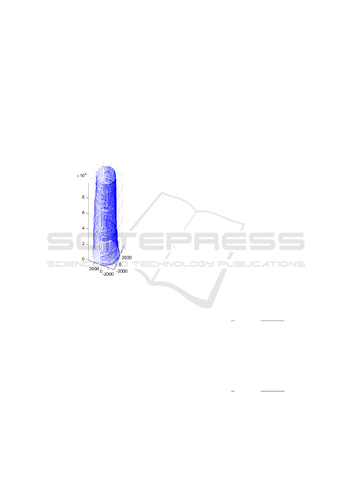
of such a log scan is presented ﬁgure 2. Each scan

can be seen as a table of dimension N

× 3, with N

the number of points, which changes from one scan

to another, with an average of 12 000 points per scan.

Each of the 3 points coordinates corresponds to one

column in the scan table.

Additionally, points, are roughly organized as el-

lipsoids which, together, span the log surface. Orig-

inally, the scans contained sections with missing el-

lipsoids, which led to poor performances of the ICP

algorithm when computing logs dissimilarities. This

was corrected by ﬁlling these empty sections with rep-

etitions of the ellipsoid which immediately precedes

them.

Figure 2: Example of a 3D full proﬁle scan of a log.

The basket of products associated with each log

was generated by the sawing simulator Optitek. The

dataset contains 19 different types of individual prod-

ucts, characterized by their length, width and thick-

ness. Therefore, the structured output vector one has

to predict is of dimension 19. It might be noticed

that no basket contains more than 5 different types of

products and that, therefore, these vectors are sparse.

For training, selection and evaluation purpose, the

dataset was randomly divided into three parts, that is,

a training set containing 600 logs, a validation set con-

taining 400 logs, and an evaluation set containing the

remaining 207 logs. The training set contains only

62 different classes, which should lead to 62 medoids

used to build features. However, most of these classes

appear only once in the dataset. Therefore, to reduce

the dimension of the input vector, composed of dis-

similarities toward these class medoids, a medoid is

considered to induce a feature only if it corresponds

to a class with more than two elements in the training

set. This reduces the dimension of the input vector to

21.

A drawback of using the ICP dissimilarity in our

case is, however, its behavior when comparing logs

of different lengths. When comparing a long log with

a short one, the value of the dissimilarity explodes

compared with the normal range of values when us-

ing short logs only. This creates unwanted but ex-

tremely high correlations between the 8 features built

from dissimilarities to shorter logs. To solve this is-

sue, these features were clipped to 3000, as is shown

in ﬁgure 3.

3.3 Evaluation Scores

As per usual, evaluation scores have to be deﬁned

to evaluate and compare the different models. Sev-

eral set of scores were introduced speciﬁcally for the

problem of evaluating sawing metamodels. It was, in-

deed, observed that in a classiﬁcation setting, classic

scores like the 0-1 score don’t take into consideration

the fact that the cost of missclassiﬁcation might vary

among different real/predicted pairs, while in a re-

gression setting, the squared error is difﬁcult to inter-

pret. Therefore, the prediction score, s

pre

, production

score, s

pro

and prediction-production score, s

pre×pro

were deﬁned by (Morin et al., 2015). Similarly, adap-

tation of the classic precision, recall and F

scores

were introduced in (Martineau et al., 2021).

First, considering that the vectors representing the

baskets of products are sparse, to let all the (0,0)

real/predicted pairs in these vectors might biased s

pre

pro

, and s

pre×pro

optimistically, all such pairs are re-

moved. Consider ˜p the length of the ﬁltered vectors.

The prediction score is then deﬁned as:

pre

(y, ˆy) =

˜p

∑

i=1

min(1,

ˆy

max(ε, y

)

), (2)

with ε a small value to avoid dividing by zero. y

and ˆy

are the i

components of the real and predicted

vectors respectively. This score can be seen as the per

product average proportion of the real basket which is

effectively predicted.

Similarly, the production score is deﬁned as:

pro

(y, ˆy) =

˜p

∑

i=1

min(1,

max(ε, ˆy

)

), (3)

and can be seen as the per product average propor-

tion of the prediction which is effectively produced.

It might be observed, however, that always pre-

dicting an empty basket of product would lead to

NCTA 2021 - 13th International Conference on Neural Computation Theory and Applications

204

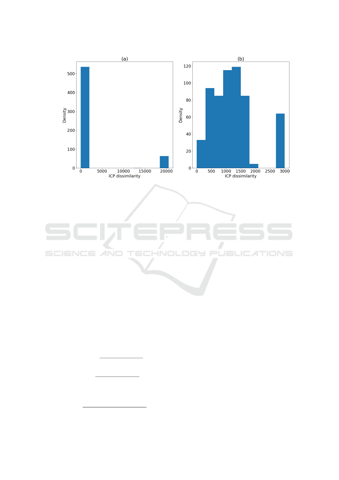
Figure 3: Histograms of dissimilarities to a short medoid. (a) corresponds to in the unclipped dissimilarities. For (b),

dissimilarities were clipped to 3000, deplacing the density peak initially around 20000 toward 3000.

a perfect production score, while predicting a bas-

ket with a very high number of each product would

lead to a perfect prediction score. These two scores

need, therefore, to be balanced inside the prediction-

production score, naturally deﬁned as:

pre×pro

= s

pre

× s

pro

. (4)

As for precision, recall and F

, they are based on

a redeﬁnition of True positives (TP), False Positives

(FP) and False Negatives (FN):

• TP is the number of lumbers which are present in

both the real and predicted basket of a log, that is,

T P(y, ˆy) =

∑

i=1

min(y

, ˆy

• FP is the number of lumbers present in the pre-

dicted basket of a log, but not in its real basket,

that is, FP(y, ˆy) =

∑

i=1

max( ˆy

− y

, 0).

• FN is the number of lumbers present in the real

basket of a log but not in its predicted basket, that

is, FP(y, ˆy) =

∑

i=1

max(y

− ˆy

, 0).

precision, recall and F1 are then classically de-

ﬁned as:

precision(y, ˆy) =

T P(y, ˆy)

T P(y, ˆy) + FP(y, ˆy)

, (5)

recall(y, ˆy) =

T P(y, ˆy)

T P(y, ˆy) + FN(y, ˆy)

, (6)

and

(y, ˆy) = 2

precision(y, ˆy)recall(y, ˆy)

precision(y, ˆy) + recall(y, ˆy)

. (7)

While these scores are estimated individually for

each log, the quantity of interest is, naturally, their

average over the evaluation dataset.

4 DESCRIPTION OF THE

PREDICTORS

Several model architectures are tested and com-

pared. These individual models are later used to build

different predictors ensembles.

4.1 Individual Models

There exists two popular methods for handling mul-

tiple outputs prediction in such a regression frame-

work. (Borchani et al., 2015) refers to them as prob-

lem transformation methods and algorithm adapta-

tion method. Problem transformation methods change

the multiple outputs problem into several single out-

put problems. In our case, it corresponds to training

one MLP for each type of lumber in the basket of

products. On the contrary, algorithm adaptation meth-

ods use algorithms designed or modiﬁed to handle si-

multaneously all the outputs. While problem trans-

formation methods use simpler models, which might

lead to better individual accuracy and smaller training

time, they cannot be expected to handle dependencies

among the outputs. Both of these strategies are tested

in this paper.

Medoid-based MLP: An Application to Wood Sawing Simulator Metamodeling

205

Table 1: Summary table of the individual models being compared in this study.

Model hidden layer size number of weights output activation

MIMO 5 224

Hyperbolic tangent

Sigmoid

Linear

Relu

MISO 2

Hyperbolic tangent

Sigmoid

Linear

4.1.1 Multiple Input, Single Output (MISO)

MISO models belong to the problem transformation

family. Different MLPs are trained separately for

each one of the 19 dimensions of the output vector.

Therefore, 19 such individual MLPs, or MLP ensem-

bles, are necessary to predict the whole vector. These

MLPs are composed of one entry layer of size 21.

The number of neurons in the single hidden layer was

ﬁxed to 2 by trials and errors. To increase it even to

3 neurons leads to a strong overﬁtting of the learning

base by the MLPs. The activation function of the hid-

den layer is always a hyperbolic tangent. However,

several common activation functions for the output

layer are compared: linear, sigmoid and hyperbolic

tangent. An inconvenient of the linear output activa-

tion is that it allows the prediction of negatives lum-

ber quantities, which have no reality in practice. Once

trained, the prediction of these networks were there-

fore clipped to 0 when negative. Since the sigmoid

and hyperbolic tangent have values between 0 and 1,

or between -1 and 1 respectively, the outputs where

scaled accordingly for training with min-max trans-

formations. These activation functions have the ad-

vantage that they constrain the inversely transformed

prediction to stay between 0 and the maximum value

encountered in the training set. A Relu activation

function was similarly tested. However, it appears in

practice that, in the MISO case, this activation leads

to null gradients extremely early during the training

process, sometimes even during the initial iteration.

The sparsity of the output and the fact that the Relu is

constant for negative values make it, indeed, possible

to initialize the network at a point where the gradient

is null. In particular, over 150 such models trained for

the different outputs, 27% run less than 5 iterations

of the optimization algorithm used before triggering a

stopping condition. A discussion about the trainabil-

ity of Relu-based NN, and the problem of dying neu-

rons, can be found in (Shin and Karniadakis, 2020).

MISO models with Relu activation are therefore not

studied further in this paper.

4.1.2 Multiple Input, Multiple Output (MIMO)

Contrary to the MISO models, MIMO belong to the

algorithm adaptation family, as all outputs are pre-

dicted simultaneously by the same MLP. Similarly to

the MISO case, the input layer is of size 21. However,

the number of neurons in the hidden layer was only

reduced to 5 neurons. Similarly to what was tested

in the MISO case, linear, sigmoid, hyperbolic tangent

and Relu activation functions are tested for the output

layer.

Table 1 summarizes the different architectures,

and in particular provides the number of weights for

each model. Since the limited size of the problem

considered allows it, all neural networks were trained

using Levenberg-Marquardt algorithm (Yu and Wil-

amowski, 2011), rather than a gradient descent. As

explained for example by these authors, this algorithm

is fast, as long as the matrix considered in its iteration

are not too big, and it has stable convergence. Initial-

ization of the networks was done using the Nguyen-

Widrow algorithm (Nguyen and Widrow, 1990).

4.2 Ensemble Selection

Creating ensembles is a commonly used method to

improve on the results of a set of predictors (as in, to

increase or minimize a chosen set of scores, for exam-

ple the MSE in this paper). In particular, NN ensem-

bles were introduced in (Hansen and Salamon, 1990).

It is based on the fact that when training multiple NN

with variations on the training method, for example

different initializations, the training of these NN will

converge toward different local minimums. Popular

methods to introduce variety into the training of ML

predictors include bagging (Breiman, 1996), boosting

(Freund et al., 1996) or the Random Subspace method

(Ho, 1998).

Additionally, numerous methods have been pro-

posed to select predictors from a set of previously

trained models. (Thomas et al., 2018) reports that

two such families of methods either perform a selec-

tion based solely on a performance score, for exam-

ple the MSE, or perform a selection based on both a

NCTA 2021 - 13th International Conference on Neural Computation Theory and Applications

206

performance scores and a diversity score. However,

when comparing two such methods on their industrial

dataset, they found no signiﬁcant advantage to the use

of a diversity based method, compared to the use of a

performance based method.

In the following of this paper, we will therefore

focus on a method to select MLPs for the ensembles

based on the MSE score only. This method proceed

as follow:

1. Evaluate the MSE of all the MLPs on a validation

set and order them from best to worst.

2. from the best to the worst model, add them to the

ensemble, and evaluate the ensemble MSE on the

validation set.

3. Select the ensemble showing the lowest MSE.

The prediction of an ensemble are here the aver-

aged predictions of its individual elements. Addition-

ally, 150 individual NN were trained with random ini-

tialization for each output of each of the MISO mod-

els, and 150 other for each of the MIMO models.

5 RESULTS AND DISCUSSION

This section presents the experimental results of our

different models, ﬁrst taken individually and later

used to build ensembles. Considering that, in practice,

a basket of products is a vector of integer, any poten-

tial negative predicted value was set to 0, and outputs

were rounded to the nearest integer. This addition-

ally favor the emergence of null outputs which play

an important role in the evaluation scores, especially

the prediction, production, and prediction-production

scores.

5.1 Individual Models

150 models where trained for each architecture. Fig-

ure 4 shows the MSE of all the trained models, eval-

uated on the validation set. In the MISO case, pre-

dictions of a complete output vector where built by

associating the predictions of the individual MISO in

training order. The ﬁrst MISO trained for all 19 out-

puts are used to generate a complete predictor, then

the second MISO trained for all 19 outputs generate a

second predictor, and so on. This ﬁgure shows, over-

all, an advantage of the Sigmoid activation function,

both for MIMO and MISO models. Their MSE are,

indeed, generally lower and present lower variation

than other architectures.

Table 2 presents the scores of the best MIMO

and MISO models with different outputs activation

Table 2: Mean evaluation scores for the different individual

models with lower MSE on the validation set, in percent,

and their asymptotic conﬁdence interval at a 95% level.

These scores are evaluated on the evaluation set. The best

scores are highlighted in bold. Scores which can’t be said to

be statistically different from the best model at a 5% level

using a Wilcoxon test are set in italic. The total training

time necessary to train all models with an architecture is

also displayed.

Model Output total training time s

pre

pro

pre×pro

precison recall F

MSE

MIMO Tanh 58395 s 84.6 ± 3.7 89.2 ± 2.9 76.3± 4.4 85.6± 3.7 81.5 ± 4.2 79.5 ± 4.3 1.03 ± 0.26

MIMO Sigmoid 6375 s 86.5 ± 3.3 89.2 ± 2.9 78.3 ± 4.4 86.8 ± 3.4 83.3 ± 3.9 81.7 ± 4.0 1.04 ± 0.33

MIMO Linear 675 s 84.7 ± 3.3 86.1 ± 3.6 73.6 ± 4.6 83.6 ± 3.9 81.2 ± 3.9 77.6 ± 4.3 1.07 ± 0.3

MIMO Relu 1005 s 87.3 ± 3.0 85.1 ± 3.9 75.0 ± 4.7 82.5 ± 4.3 83.8 ± 3.7 77.9 ± 4.5 1.02 ± 0.29

MISO Tanh 1924 s 85.8 ± 3.4 90.9 ± 2.5 79.4 ± 4.2 88.0 ± 3.3 82.6 ± 4.0 82.4 ± 4.0 0.913 ± 0.27

MISO sigmoid 465 s 87.2 ± 3.1 91.9 ± 2.5 81.6 ± 4.0 89.0 ± 3.3 84.5 ± 3.7 84.7 ± 3.7 0.865 ± 0.29

MISO Linear 186 s 86.4 ± 3.0 87.4 ± 3.4 76.7 ± 4.4 84.9 ± 3.8 82.7 ± 3.7 80.2 ± 4.1 0.957 ± 0.280

Medoid-based MLP: An Application to Wood Sawing Simulator Metamodeling

207

Figure 4: Boxplots of the MSE, estimated over the validation set, of the 150 models trained for each architecture. Prediction

where inversely scaled for models having sigmoid or tanh output, to allow comparison.

functions, and their asymptotic 95% conﬁdence in-

tervals. These scores are evaluated on the evaluation

set. These models were selected as being the ones

with the lowest squared error over the validation set,

among the 150 models with same architecture. In

particular, in the MISO case, a complete prediction

of the output vector is done by concatenation of the

MISO which perform the best on their respective in-

dividual output. This table also displays, for each ar-

chitecture, the total time needed to train all the 150

models. The models were implemented in Python

and trained on an intel Core i7 vPRO 10

generation

CPU at 2.70GHz. Matrix operations are performed

with the library Numpy. It appears than on the dataset

used in this study, the MISO model with sigmoid out-

put performs best. In particular, it has the highest

prediction-production score and F

and lowest MSE.

It might be noticed that, similarly, the model with

higher prediction-production score and F

among the

MIMO models only is the one with sigmoid output.

While the selected models with Tanh architecture per-

form relatively well on the evaluation set, however,

the results from ﬁgure 4 do not encourage the use of

this particular activation function.

Additionally, one should be careful that these dif-

ferences in score, despite appearing important, are not

always statistically signiﬁcant. This is partly due to

the high variability of the scores, and extensive tests

on a larger dataset would be required to conclude on a

difference. Here, in particular, when comparing the F

scores of the MISO sigmoid models with the scores of

all the other selected models using Wilcoxon signed

rank test, it cannot be said to be statistically different,

at a 5% level, from the MISO model with hyperbolic

tangent output (p-value at 18.9%) and MIMO model

with sigmoid output (p-value at 9.2%). However, both

the MIMO and MISO models with linear or Relu acti-

vation perform relatively poorly compared with mod-

els of the same family.

It may be noticed that MISO models are, in aver-

age, faster to train than MIMO models as they contain

less parameters. In particular, a MISO sigmoid model

is, in average, more than 200 times faster to train than

a MIMO sigmoid. Even when considering that 19

such networks have to be trained to perform a predic-

tion of the full basket, this is an improvement. Inter-

estingly, models with hyperbolic tangent output are

relatively slow to train, as it appears in practice that

they need more iterations of the levenberg-Marquardt

algorithm before triggering a stopping condition.

5.2 Ensemble

Table 3 presents the averaged scores over the eval-

uation database of ensembles based on MLPs with

different architectures. While the ensembles seem

to improve upon the scores of several models, these

differences are nearly never statistically signiﬁcant,

at a 5% level, under Wilcoxon signed ranks test. In

particular, the scores of the MISO sigmoid ensemble

are never statistically different from the scores of the

previously selected MISO sigmoid model, despite ap-

pearing even slightly lower than the scores of the in-

dividual models.

Concerning the size of the ensembles, the fact that

the MISOs appears to need more models is due to the

fact that 19 ensembles are needed to make a predic-

tion of the complete output vector, and that all of that

all of them are counted in table 3. As was observed

in (Thomas et al., 2018), this method of building en-

sembles leads to parsimonious ensembles, containing

only a small number of individual models. This is

NCTA 2021 - 13th International Conference on Neural Computation Theory and Applications

208

Table 3: Mean evaluation scores for the different ensembles

on the evaluation set, in percent, and there asymptotic conﬁ-

dence interval at a 95% level. The number of MLPs used in

the ensembles are also displayed. The best scores are high-

lighted in bold. Scores statistically different from the ones

of the previously selected individual model are set in italic.

Model Output size s

pre

pro

pre×pro

precison recall F

MSE

MIMO Tanh 16 85.9 ± 3.5 91.0 ± 2.5 79.3 ± 4.2 88.5 ± 3.2 83.0 ± 4.0 82.8 ± 3.9 0.942 ± 3.0

MIMO Sigmoid 3 87.5 ± 3.0 89.5 ± 2.9 79.8 ± 4.1 87.2 ± 3.4 84.0 ± 3.7 83.0 ± 3.8 0.922 ± 3.1

MIMO Linear 4 85.7 ± 3.1 83.9 ± 4.0 72.4 ± 4.8 81.4 ± 4.3 82.2 ± 3.8 76.2 ± 4.5 1.072 ± 0.299

MIMO Relu 16 85.2 ± 3.2 90.3 ± 2.9 78.1 ± 4.3 87.5 ± 3.5 81.7 ± 3.9 81.5 ± 3.9 0.976 ± 0.295

MISO Tanh 218 86.4 ± 3.4 91.5 ± 2.3 80.3 ± 4.1 88.7 ± 3.1 83.6 ± 3.9 83.5 ± 3.8 0.835 ± 0.241

MISO sigmoid 60 86.8 ± 3.2 92.3 ± 2.3 81.5 ± 4.0 89.3 ± 3.1 84.1 ± 3.7 84.9 ± 3.6 0.870 ± 0.249

MISO Linear 44 86.6 ± 3.0 86.4 ± 3.5 75.9 ± 4.5 84.0 ± 3.9 82.7 ± 3.7 79.6 ± 4.1 0.976 ± 0.280

particularly the case of the models with sigmoid and

linear outputs.

6 CONCLUSION

The set of features based on dissimilarities to medoids

used to train MLPs in this study gives satisfactory re-

sults. This study furthermore compares several MLP

architectures to the task of predicting baskets of prod-

ucts from 3D scans of wood logs. It appears that using

an output activation function constraining the individ-

ual outputs in a certain value range leads to better

evaluations scores, as the MLPs cannot predict un-

realistic values. Therefore, both MIMO and MISO

with sigmoid outputs work well and can be trained

in reasonable time, with MISO performing seemingly

better on our dataset. This is of particular interest

when considering the fact that the sawmill conﬁgu-

ration used in this paper processes a relatively small

number of products. For example, (Morin et al., 2020)

considers sawmills with as much as 83 products. The

fact that ensembles barely increase the performances

of the models is however surprising and may raise

doubts on the possibility to consistently increase fur-

ther the evaluation scores, at least when using only

this set of medoid-based features.

Additionally, it appears that one should be ex-

tremely careful when working on this problem to

avoid overﬁtting of the training database.

While in this paper, the features were selected

as dissimilarities to class medoids, other logs could

have been selected has references. To use meta-

heuristics like genetic algorithms or other feature se-

lection methods during training time to select these

logs might appears as a promising research direction

for future works. Similarly, other classic ML algo-

rithms, such as Random forest, will be investigated.

ACKNOWLEDGEMENTS

The authors gratefully acknowledge the ﬁnancial sup-

port of the ANR-20-THIA-0010-01 Projet LOR-AI

(lorraine intellgence artiﬁcielle) and r

egion Grand

EST. We are also extremely grateful to FPInnovation

who gathered and processed the dataset we are work-

ing with.

REFERENCES

Besl, P. J. and McKay, N. D. (1992). A method for regis-

tration of 3-d shapes. IEEE Transactions on Pattern

Analysis and Machine Intelligence, 14(2):239–256.

Borchani, H., Varando, G., Bielza, C., and Larranaga, P.

(2015). A survey on multi-output regression. Wiley

Interdisciplinary Reviews: Data Mining and Knowl-

edge Discovery, 5(5):216–233.

Medoid-based MLP: An Application to Wood Sawing Simulator Metamodeling

209

Breiman, L. (1996). Bagging predictors. Machine learning,

24(2):123–140.

Cazzanti, L. (2009). Similarity Discriminant Analysis.

Chabanet, S., Thomas, P., El-Haouzi, H. B., Morin, M., and

Gaudreault, J. (2021). A knn approach based on icp

metrics for 3d scans matching: an application to the

sawing process. In 17th IFAC Symposium on Infor-

mation Control Problems in Manufacturing, INCOM

2021.

Del Frate, F. and Solimini, D. (2004). On neural network

algorithms for retrieving forest biomass from sar data.

IEEE Transactions on Geoscience and Remote Sens-

ing, 42(1):24–34.

Duin, R. P. and Pekalska, E. (2009). The dissimilarity rep-

resentation for pattern recognition: a tutorial. In Tech-

nical Report.

Freund, Y., Schapire, R. E., et al. (1996). Experiments with

a new boosting algorithm. In icml, volume 96, pages

148–156. Citeseer.

Goulet, P. (2006). Optitek: User’s manual.

Hansen, L. K. and Salamon, P. (1990). Neural network en-

sembles. IEEE transactions on pattern analysis and

machine intelligence, 12(10):993–1001.

Ho, T. K. (1998). The random subspace method for con-

structing decision forests. IEEE transactions on pat-

tern analysis and machine intelligence, 20(8):832–

844.

Martineau, V., Morin, M., Gaudreault, J., Thomas, P., and

Bril El-Haouzi, H. (2021). Neural network architec-

tures and feature extraction for lumber production pre-

diction. In The 34th Canadian Conference on Artiﬁ-

cial Intelligence. Springer.

Morin, M., Gaudreault, J., Brotherton, E., Paradis, F., Rol-

land, A., Wery, J., and Laviolette, F. (2020). Machine

learning-based models of sawmills for better wood al-

location planning. International Journal of Produc-

tion Economics, 222:107508.

Morin, M., Paradis, F., Rolland, A., Wery, J., Laviolette,

F., and Laviolette, F. (2015). Machine learning-based

metamodels for sawing simulation. In 2015 Win-

ter Simulation Conference (WSC), pages 2160–2171.

IEEE.

Morneau-Pereira, M., Arabi, M., Gaudreault, J., Nourelfath,

M., and Ouhimmou, M. (2014). An optimization

and simulation framework for integrated tactical plan-

ning of wood harvesting operations, wood allocation

and lumber production. In MOSIM 2014, 10eme

Conf

erence Francophone de Mod

elisation, Optimisa-

tion et Simulation.

Nguyen, D. and Widrow, B. (1990). Improving the learning

speed of 2-layer neural networks by choosing initial

values of the adaptive weights. In 1990 IJCNN Inter-

national Joint Conference on Neural Networks, pages

21–26. IEEE.

Pekalska, E., Duin, R. P., and Pacl

ık, P. (2006). Prototype

selection for dissimilarity-based classiﬁers. Pattern

Recognition, 39(2):189–208.

Qi, C. R., Su, H., Mo, K., and Guibas, L. J. (2017). Point-

net: Deep learning on point sets for 3d classiﬁcation

and segmentation. In Proceedings of the IEEE con-

ference on computer vision and pattern recognition,

pages 652–660.

Schleif, F.-M. and Tino, P. (2015). Indeﬁnite prox-

imity learning: A review. Neural Computation,

27(10):2039–2096.

Selma, C., El Haouzi, H. B., Thomas, P., Gaudreault, J.,

and Morin, M. (2018). An iterative closest point

method for measuring the level of similarity of 3d

log scans in wood industry. In Service Orientation in

Holonic and Multi-Agent Manufacturing, pages 433–

444. Springer.

Shin, Y. and Karniadakis, G. E. (2020). Trainability of relu

networks and data-dependent initialization. Journal of

Machine Learning for Modeling and Computing, 1(1).

Sylvain, J.-D., Drolet, G., and Brown, N. (2019). Mapping

dead forest cover using a deep convolutional neural

network and digital aerial photography. ISPRS Jour-

nal of Photogrammetry and Remote Sensing, 156:14–

26.

Thomas, P., El Haouzi, H. B., Suhner, M.-C., Thomas, A.,

Zimmermann, E., and Noyel, M. (2018). Using a clas-

siﬁer ensemble for proactive quality monitoring and

control: The impact of the choice of classiﬁers types,

selection criterion, and fusion process. Computers in

Industry, 99:193–204.

Thomas, P. and Thomas, A. (2011). Multilayer percep-

tron for simulation models reduction: Application to

a sawmill workshop. Engineering Applications of Ar-

tiﬁcial Intelligence, 24(4):646–657.

Todoroki, C. et al. (1990). Autosaw system for sawing sim-

ulation. New Zealand Journal of Forestry Science,

20(3):332–348.

Wenshu, L., Lijun, S., and Jinzhuo, W. (2015). Study on

wood board defect detection based on artiﬁcial neural

network. The Open Automation and Control Systems

Journal, 7(1).

Wery, J., Gaudreault, J., Thomas, A., and Marier, P. (2018).

Simulation-optimisation based framework for sales

and operations planning taking into account new prod-

ucts opportunities in a co-production context. Com-

puters in industry, 94:41–51.

Yu, H. and Wilamowski, B. M. (2011). Levenberg-

marquardt training. Industrial electronics handbook,

5(12):1.

Zhang, B., Zhao, L., and Zhang, X. (2020). Three-

dimensional convolutional neural network model for

tree species classiﬁcation using airborne hyperspectral

images. Remote Sensing of Environment, 247:111938.

NCTA 2021 - 13th International Conference on Neural Computation Theory and Applications

210