Matching Entities from Multiple Sources with Hierarchical

Agglomerative Clustering

Alieh Saeedi

1,2 a

, Lucie David

1 b

and Erhard Rahm

1,2 c

University of Leipzig, Germany

ScaDS.AI Dresden/Leipzig, Germany

Keywords:

Entity Resolution, Hierarchical Agglomerative Clustering , Multi-source ER, MSCD-HAC.

Abstract:

We propose extensions to Hierarchical Agglomerative Clustering (HAC) to match and cluster entities from

multiple sources that can be either duplicate-free or dirty. The proposed scheme is comparatively evaluated

against standard HAC as well as other entity clustering approaches concerning efﬁciency and efﬁcacy criteria.

All proposed algorithms can be run in parallel on a distributed cluster to improve scalability to large data

volumes. The evaluation with diverse datasets shows that the new approach can utilize duplicate-free sources

and achieves better match quality than previous methods.

1 INTRODUCTION

Entity Resolution (ER) is the task of identifying enti-

ties in a single or several data sources that represent

the same real-world entity (e.g., a speciﬁc costumer or

product). ER is of key importance for improving data

quality and integrating data from multiple sources.

Most previous ER solutions perform ER process be-

tween at most two sources. By raising the number of

sources (> 2), data heterogeneity as well as the vari-

ance in data quality is increased. Multi-source ER,

i.e. ﬁnding matching entities in an arbitrary number

of sources, is thus a challenging task.

Multi-source ER works in two main steps. In the

ﬁrst step, similar pairs of entities inside or across data

sources are determined. Then in the next step match-

ing entities are grouped within a cluster. We refer to

the ﬁrst step as linking and record its output in a sim-

ilarity graph where each vertex represents an entity

and each edge a similarity relationship between two

entities. Edges maintain similarity values reﬂecting

the match probability and only edges with a similarity

above a certain threshold are recorded. Such a simi-

larity graph is the input of the clustering phase.

Most previous ER clustering approaches clus-

ter entities of a single source [Hassanzadeh et al.,

2009, Saeedi et al., 2017], or of multiple duplicate-

https://orcid.org/0000-0002-1066-1959

https://orcid.org/0000-0002-5751-696X

https://orcid.org/0000-0002-2665-1114

free sources [Nentwig et al., 2016,Saeedi et al., 2018].

We recently started to address the more general multi-

source case with a combination of duplicate-free and

dirty (containing duplicates) sources [Lerm et al.,

2021]. Duplicate-free sources imply an important

constraint that can be utilized for improved cluster

quality, namely that any cluster of matching entities

can include at most one entity of any duplicate-free

source. While our previous Multi-Source Clean/Dirty

(MSCD) clustering approach utilized afﬁnity propa-

gation clustering [Lerm et al., 2021] we investigate

here the use of Hierarchical Agglomerative Cluster-

ing (HAC) for MSCD entity clustering. The special

cases with only dirty or only clean sources are also

supported.

We make the following contributions:

• We propose the MSCD-HAC algorithm for multi-

source entity clustering with a combination of

clean (duplicate-free) and dirty sources. The clus-

ters to merge in the next iteration can be selected

based on the maximal, minimal, or average sim-

ilarity of their cluster members. The approach

utilizes the clustering constraint for clean sources

and can optionally ignore so-called weak links in

the similarity graph for improved quality and run-

time.

• We provide a parallel implementation of the ap-

proach on top of Apache Flink for improved run-

time and scalability.

Saeedi, A., David, L. and Rahm, E.

Matching Entities from Multiple Sources with Hierarchical Agglomerative Clustering.

DOI: 10.5220/0010649600003064

In Proceedings of the 13th International Joint Conference on Knowledge Discovery, Knowledge Engineering and Knowledge Management (IC3K 2021) - Volume 2: KEOD, pages 40-50

ISBN: 978-989-758-533-3; ISSN: 2184-3228

• We perform a comprehensive evaluation of match

quality, runtime and scalability of the new ap-

proaches for different datasets and compare them

with previous clustering schemes. The evalua-

tion shows that the new approach achieves better

match quality than previous approaches.

After a discussion of related work, we introduce

the hierarchical cluster analysis in Section 3. Sec-

tion 4 presents the new clustering method MSCD-

HAC in detail as well as the parallel version. In Sec-

tion 5 we present our evaluation before we conclude.

2 RELATED WORK

A wide range of general purpose clustering schemes

have been used to group matches in a single source.

Hassanzadeh et al. [Hassanzadeh et al., 2009] give

a comprehensive comparative evaluation of them for

single source ER. Distributed implementations of

these approaches for multi-source ER have been pre-

sented and comparatively evaluated in [Saeedi et al.,

2017]. Multi-source clustering schemes exclusively

developed for clean sources [Nentwig et al., 2016,

Saeedi et al., 2018] could obtain superior results com-

pared to general purpose clustering algorithms. Re-

cently, Lerm et al. [Lerm et al., 2021] extended afﬁn-

ity propagation clustering for multi-source clustering,

which is able to consider a combination of dirty and

clean sources as input. The method tends to form

many small clusters and achieves a high precision but

at the cost of relatively low recall, indicating room for

improvement.

Hierarchical clustering is a popular clustering ap-

proach that has also been employed for ER [Mamun

et al., 2016]. Recently, Yan et al. [Yan et al., 2020]

propose a modiﬁed hierarchical clustering that aims

at avoiding so-called hard conﬂicts introduced by sys-

tematically missing information in different sources.

Many approaches try to make hierarchical clustering

faster, which is inherently iterative and thus sequen-

tial. Some approaches reduce the hierarchical clus-

tering to the problem of creating the Minimum Span-

ning Tree (MST) [Dahlhaus, 2000] while others ap-

proximate the results by utilizing Locality-Sensitive

Hashing (LSH) [Koga et al., 2007]. Another option

considered is to partition data evenly on processing

nodes before performing clustering [Hendrix et al.,

2012,Jin et al., 2015,Dash et al., 2007]. Furthermore,

a method based on the concept of Reciprocal Nearest

Neighbors (RNN) that ﬁts graph clustering can be ap-

plied [Murtagh and Contreras, 2012, Murtagh, 1983].

In this work, we extend the usage of hierarchical

clustering for efﬁcient and effective clustering of en-

tities from a combination of arbitrary portion of clean

and dirty sources. We further enable the algorithm to

improve the ﬁnal results by removing potential false

links (weak links) in a preprocessing step. To im-

prove scalability, the parallel variant is implemented

based on the RNN concept using scatter-gather itera-

tions [Junghanns et al., 2017].

3 HIERARCHICAL CLUSTER

ANALYSIS

Hierarchical Cluster Analysis (HCA) [Ward Jr, 1963]

comprises clustering algorithms that pursue building

a hierarchy of clusters where a higher-level cluster

combines two clusters of the level and this construc-

tion principle is recursively applied leading to a hier-

archy of clusters. The hierarchies can be formed in a

bottom-up or top-down manner. The bottom-up ap-

proach known as agglomerative merges the two most

similar clusters as one cluster that is moved up the hi-

erarchy. In contrast, the top-down approach is divisive

and initially assumes all entities build a single cluster.

Then it performs splitting this cluster into two clusters

in a recursive manner. Each splitted cluster moves one

step down the hierarchy [Rokach and Maimon, 2005].

The results of hierarchical clustering form a bi-

nary tree that can be visualized as a dendrogram

[Nielsen, 2016]. The decision on merging (in agglom-

erative approach) or splitting (in divisive approach) is

based on a greedy strategy [Murtagh and Contreras,

2012]. Due to the fact that there are 2

possibilities

for splitting a set of n entities, the divisive approach is

not usually feasible for practical applications [Kauf-

man and Rousseeuw, 1990]. Therefore, we focus on

Hierarchical Agglomerative Clustering (HAC) in this

paper.

The agglomerative approach initially assumes that

each entity forms a cluster and it then selects and

merges the two most similar clusters as one cluster.

The process of selecting and merging continues in an

iterative way until a stopping condition is satisﬁed.

The hierarchical clustering scheme may lead into to-

tally different clustering results depending on the ap-

proach to determine the similarity between clusters

and depending on the stopping condition [Kaufman

and Rousseeuw, 1990]. The rule that determines the

most similar clusters is known as linkage strategy.

Considering two clusters c

and c

, the similarity

of them is denoted as Sim

. The similarity of a pair

of clusters is a function of similarity of their members

(entities). The similarity of two cluster members

(entities) e

and e

are denoted as sim(e

). In this

paper, we implement and evaluate three commonly

Matching Entities from Multiple Sources with Hierarchical Agglomerative Clustering

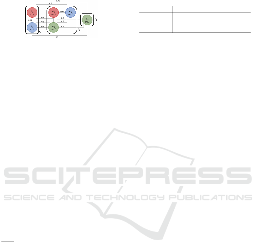
Figure 1: Hierarchical clustering example.

used approaches for computing Sim

that offer low

computation cost. The three linkage strategies [Kauf-

man and Rousseeuw, 1990] are deﬁned as follows:

S-LINK (Single-Linkage): is referred to as the

nearest-neighbor strategy. It determines the cluster

similarity based on the two closest entities from

each cluster, i.e., considering the maximal similarity

between members of the two clusters. The single

linkage implies that S im

= max{sim(e

)}

where e

∈ c

and e

∈ c

. This is an optimistic

approach that ignores that there may be dissimilar

members in the two clusters, which might help to

improve recall at the expense of precision.

C-LINK (Complete-Linkage): is known as the

furthest-neighbor strategy. The two most dissimilar

entities of two cluster determine the inter-cluster

similarity, i.e. based on the minimum similarity

between members of the two clusters. The complete

linkage implies that Sim

= min{sim(e

)}

where e

∈ c

and e

∈ c

. This is a conservative

or pessimistic approach that might help to improve

precision at the expense of recall.

A-LINK (Average-Linkage): deﬁnes the

cluster similarity as the average similarity

of the entities of two clusters: Sim

|·|c

∑

∈c

sim(e

The application of HAC results in a set of clus-

terings, one at each level of the cluster hierarchy.

Determining the optimal clustering from the hier-

archy is not a trivial decision with large datasets.

Therefore, metrics such as number of clusters or a

minimum merge threshold are used as the stopping

criteria. Due to the fact that the number of output

clusters are not predeﬁned in ER applications, we

use the merge threshold (T ) as stopping condition.

Hence, the algorithm stops as soon as there is no

further pair of clusters whose similarity is exceeding

the merge threshold.

Figure 1 shows an example of three clusters along

with the similarities between entities (from the sim-

ilarity graph). Table 1 lists the inter-cluster simi-

larity of all possible cluster pairs for our three link-

Table 1: Linkage types.

Cluster pair S-LINK C-LINK A-LINK

0.80 0.00 0.48

0.75 0.50 0.62

0.60 0.60 0.40

vspace0.15cm

ages types. For S-LINK (ﬁrst column), the most sim-

ilar cluster pair is {c

, c

} because the maximum

link between these clusters has the highest similar-

ity compared with the two other cluster pairs. For

C-LINK (second column) we have cluster similarity

0 for {c

, c

} due to the missing similarity links for

cluster members. Thus c

and c

with inter-cluster

similarity 0.6 are the most similar clusters. For A-

LINK, the cluster pair {c

, c

} has the highest aver-

age similarity. Hence, we have different merge deci-

sions for each of the three strategies.

4 MULTI-SOURCE

HIERARCHICAL CLUSTERING

In this section, we initially deﬁne some key concepts,

and then we explain the newly proposed approaches.

4.1 Concepts

Similarity Graph: A similarity graph G= (V , E)

is a graph in which vertices of V represent entities

and edges of E are links between matching entities.

There is no direct link between entities of the same

duplicate-free source. Edges have a property for the

similarity value (real number in the interval [0,1]) in-

dicating the degree of similarity.

Clean/Dirty Data Source: A data source without du-

plicate entities is referred to as clean, while sources

that may contain duplicate entities are called dirty.

There is no need to perform linking between entities

of a clean source so that there are no links between

cluster members (in different clusters) of the same

clean source. Assuming that in our running exam-

ple (Figure 1) the sources X (colored in red) and Y

(colored in blue) are clean explains why there is no

similarity link between red entities and between blue

entities (similarity 0).

Source Consistent Cluster: If the source X is

duplicate-free, all clusters must contain at most one

entity form source X. The cluster containing at most

one entity from a clean data source is called source-

consistent. For example, in Figure 1, all three clusters

are source-consistent. However, merging cluster pairs

, c

} will violate source consistency because the

KEOD 2021 - 13th International Conference on Knowledge Engineering and Ontology Development

merged cluster would contain two entities from the

clean sources X and Y .

Weak Link: If a link l connects entities of two clean

sources and is not the maximum link from both sides

is called a weak link. In Figure 1, entity e

from

source X is connected through a weak link with sim-

ilarity value 0.8 to e

from source Y, because both e

and e

are connected to other entities from sources Y

and X respectively with higher similarity values than

0.8.

Reciprocal Nearest Neighbour (RNN): If entity e

the nearest neighbour of entity e

(NN(e

) = e

) and

vice versa (NN(e

) = e

), then e

and e

are reciprocal

nearest neighbours. In [Saeedi et al., 2018] such links

have been called strong links.

4.2 MSCD HAC

Performing ER for a mixed collection of clean

and dirty data sources requires determining source-

consistent clusters as the ﬁnal output. Therefore, the

ER pipeline should take clean sources into account in

both linking and clustering phases. Hence, the link-

ing phase does not create similarity links between

entities of the same clean source. However, the in-

direct connections (transitive closures) can still lead

to source-inconsistent clusters. To address this issue,

we propose an extension to hierarchical agglomera-

tive clustering called Multi-Source Clean/Dirty HAC

(MSCD-HAC). The proposed algorithm aims at clus-

tering datasets of combined clean and dirty sources.

Our extension to HAC introduces the following con-

tributions:

1. When picking the most similar cluster pair, the al-

gorithm checks whether merging them would lead

to a source inconsistent cluster. Such pairs are ig-

nored to ensure that only source-consistent clus-

ters are determined. If the source consistency con-

straint is not satisﬁed, then the pair is removed

from the candidate pairs set and thus the algo-

rithm skips computing the inter-cluster similarity

of them. For our running example (Figure 1),

merging clusters c

and c

for all linking strate-

gies would thus be forbidden under the assump-

tion that X and Y are clean sources.

2. When there are several clean sources, the al-

gorithm can remove weak inter-links of clean

sources in order to improve output quality. When

this option is chosen (by a parameter), a similar-

ity graph with removed weak links is processed

for clustering. For the example of Figure 1, ignor-

ing the weak link between entities e

and e

would

decrease the maximal similarity between clusters

Algorithm 1: MSCD-HAC.

Input: G(V , E), T , linkage, weakFlag, S

Output: Cluster Set CS

1 if weakFlag then

2 G(V , E

) ← removeWeakLinks(G(V , E),

3 end

4 CS ← initializeClusters(V )

5 do

6 sim

max

← 0

7 candidatePair ← {}

8 foreach c

∈ C S do

9 if isSourceConsistent(c

, S )

then

10 sim ← computeSim(c

,linkage)

11 if sim > sim

max

then

12 sim

max

← sim

13 candidatePair ← c

14 end

15 end

16 end

17 if sim

max

> T then

18 merge(candidatePair)

19 CS ← update(CS)

20 end

21 while sim

max

> T ;

and c

from 0.8 to 0.7. Therefore, S-LINK does

not decide on merging them.

The pseudocode of MSCD-HAC is shown in Al-

gorithm 1. The input of the algorithm is a similarity

graph G in which the vertices V represent entities and

each edge in the edges E connects two similar entities

and stores the similarity value of them. Further input

parameters are the stopping merge threshold T , link-

age strategy, weak link strategy weakFlag, and the set

of clean sources S. The algorithm guarantees to create

a set of source-consistent clusters CS as output. If the

weak link strategy is selected, weak links are removed

prior to performing the clustering process (lines 1-2).

As for the basic hierarchical agglomerative clustering,

the algorithm ﬁrst initializes the output cluster set C S

by assuming each entity as a cluster (line 4). Then it

iterates over all cluster pairs in CS (line 8). If merging

a cluster pair would lead to a source-consistent cluster

(line 9), the inter-cluster similarity of the pair is com-

puted using the linkage method in line 10. The pair

with the maximum similarity is considered as candi-

date pair for merging (lines 11-14) and if the similar-

ity of candidate pair (sim

max

) is higher than T , then

the clusters of the candidate pair are merged, and the

cluster set is updated (lines 17-20). The iterative algo-

rithm terminates when sim

max

is lower than the mini-

mum threshold T (line 21).

Matching Entities from Multiple Sources with Hierarchical Agglomerative Clustering

Algorithm 2: Parallel MSCD-HAC.

Input: G(V , E), T , linkage, weakFlag, S

Output: Cluster Set CS

1 if weakFlag then

2 G(V , E

) ← removeWeakLinks(G(V , E),

3 end

4 CS ← initializeClusters(V )

5 do

6 isChanged ← false

7 foreach c

∈ C S in Parallel do

8 c

← findConsistentNN(c

, T , S)

9 if c

6= Null then

10 if findNN(c

) = c

then

11 merge(c

, c

)

12 CS ← update(CS)

13 isChanged ← true

14 end

15 end

16 end

17 while isChanged

4.3 Parallel Approach

For parallelizing our approaches, we follow the con-

cept of Reciprocal Nearest Neighbour (RNN) which

has been used for parallel graph clustering algorithms

including HAC [Murtagh and Contreras, 2012] and

Center clustering [Saeedi et al., 2017]. If two clus-

ters are both at the same time the nearest neighbor of

each other (deﬁned in Section 4.1), it means they are

the two most similar clusters that can be merged with

each other. This is utilized in our parallel MSCD-

HAC algorithm shown in Algorithm 2. The input and

output are the same as for the sequential MSCD-HAC

(Algorithm 1). Similar to the sequential algorithm in

lines 1-3 weak links are removed and cluster set ini-

tialization is done (line 4). Then for each cluster c

in the cluster set CS the nearest neighbour which sat-

isﬁes the source consistency constraint is determined

(line 7-8). If any source-consistent nearest neighbour

is found (line 9) and the nearest neighbour of c

, then c

and c

are assumed as RNN (line 10) and

thus will be merged and the CS is updated (lines 11-

12). Any occurring merge represents a change in the

cluster set C S which sets the isChanged ﬂag as true

(line 13). The iterative algorithms terminates when no

change is possible in the CS (line 17).

The algorithm is implemented on top of Apache

Flink framework using the Gelly library for parallel

graph processing. Each clustered vertex stores the

clusterID as a vertex property so that vertices with the

same clusterID belong to the same cluster. In order

to facilitate computing inter-cluster similarity and up-

dating cluster information, each cluster is represented

by a center vertex which maintains all cluster infor-

mation. The center vertex is chosen randomly and

stores the list of cluster members, the list of neighbour

centers, the list of links to the neighbour centers, and

the list of data sources of the members. We use the

scatter-gather iteration processing of Gelly that pro-

vide sending messages from center vertex to any tar-

get vertex such as neighbor centers and cluster mem-

bers. For merging two clusters, one cluster accepts

the clusterID and center of the other cluster. Then

all lists of the center are updated. Each iteration of

the algorithm consists of four supersteps explained as

follows:

1. During the ﬁrst scatter-gather step the source-

consistent RNNs are found. In addition, the cen-

ter status of one cluster center in each RNN is re-

moved.

2. The old centers (vertices that lost their center sta-

tus in the previous superstep) now produce the fol-

lowing messages to complete the cluster merge:

one for each cluster member informing it about

the new cluster center and clusterID, one for the

new center including the new cluster members,

and one for each neighbor including the new cen-

terID. In the gather step vertices that receive any

message from the old center update their informa-

tion. The neighbor centers can update their edges

accordingly so that all edges in the edge list are

only connecting center vertices.

3. Now that all edges are adjusted, the old center ver-

tices produce messages for their new cluster cen-

ters including all their neighbors and correspond-

ing link values.

4. In the last step the nearest neighbor vertices are

recalculated. If the similarity to the nearest neigh-

bour is less than the stopping threshold, the vertex

will not produce any messages during the follow-

ing phase. Thus, after each round of four itera-

tions the number of active vertices as well as the

number of clusters decreases.

5 EVALUATION

We now evaluate the effectiveness and efﬁciency of

the proposed clustering approaches and provide a

comparison to basic HAC and previous clustering

schemes. We ﬁrst describe the used datasets from four

domains. We then analyze comparatively the effec-

tiveness of the proposed algorithm. Finally, we eval-

uate runtime performance and scalability.

KEOD 2021 - 13th International Conference on Knowledge Engineering and Ontology Development

5.1 Datasets and Conﬁguration Setup

The new approaches are evaluated with four multi-

source datasets of clean sources (MSC) from four

different domains (geographical points, music, per-

sons, and camera products) and eight datasets of

clean and dirty sources (MSCD) from one domain

(camera products). Table 2 shows the main char-

acteristics of the datasets

speciﬁcally the number

of sources and the number of entities. The MSCD

datasets are derived from the camera dataset of the

ACM SIGMOD 2020 Programming Contest

. Ta-

ble 3 lists the sources, the size of each source and

the number of duplicates in each source in camera

dataset. We created eight different combinations of

clean and dirty sources (listed in Table 4) and named

each one according to the percentage of entities from

clean sources, so that DS-C0 is composed of only

dirty sources while DS-C100 is a dataset of all clean

sources.

All datasets have been used in previous studies as

well. Similarly, the blocking and matching conﬁgura-

tions for MSC (listed in Table 5) and MSCD datasets

correspond to the ones in previous studies [Lerm

et al., 2021]. For the camera dataset, the manufacturer

name, a list of model names, manufacturer part num-

ber (mpn), European article number (ean), digital and

optical zoom, camera dimensions, weight, product

code, sensor type, price and resolution from the het-

erogeneous product speciﬁcations are extracted. Then

standard blocking with a combined key of manufac-

turer name and model number is applied to reduce the

number of comparisons. Within these blocks, all pairs

with exactly the same model name, mpn or ean are

classiﬁed as matches. The similarity value assigned to

each matched pair is determined from a weighted av-

erage of the character-3Gram Dice similarity of string

values and a numerical similarity of numerical values

(within a maximal distance of 30%).

5.2 ER Quality of Clustering

Algorithms

To evaluate the ER quality of our approaches we use

the standard metrics precision, recall and their har-

monic mean, F-Measure. These metrics are deter-

mined by comparing the computed match pairs with

the ground truth.

https://dbs.uni-leipzig.de/de/research/projects/

object matching benchmark datasets for entity resolution

http://www.inf.uniroma3.it/db/sigmod2020contest/

index.html

We removed the sources www.alibaba.com, because it

mostly contained non-camera entities.

Table 2: Overview of evaluation datasets.

Domain Entity properties #entity #src

DS-G geography label, longitude, 3,054 4

(MSC) latitude

DS-M music artist, title, 19,375 5

(MSC) album, year, length

DS-P1 persons name, surname, 5,000,000 5

DS-P2 (MSC) suburb, postcode 10,000,000 10

DS-C camera heterogenous 21,023 23

(MSCD) key-value pairs

Table 3: DS-C.

ID #entity dedup.

1 358 244

2 198 94

3 832 630

4 118 56

5 120 59

6 164 163

7 14,009 3,255

8 190 75

9 118 47

10 130 69

11 895 578

12 181 137

13 102 64

14 347 279

15 211 126

16 327 282

17 366 325

18 740 475

19 516 334

20 630 556

21 129 73

22 195 115

23 147 87

sum 21,023 8,123

Table 4: MSCD datasets.

Name %cln

cln

#cln

#dirt

DS-C0 0 0 21,023

DS-C26 26

1-6,

8-23

4,868 14,009

DS-C32 32 7 3,255 7,014

DS-C50 50

7, 18,

19,20,

22, 23

4,822 4,786

DS-

C62A

1, 4, 6

7, 9, 11,

13, 15,

17, 19, 20

5,748 3,536

DS-

C62B

2, 3, 5,

7, 8, 10,

12, 14,

16, 18,

21-23

5,630 3,478

DS-C80 80

1-12

14-18

6,894 1,719

DS-

C100

100 1-23 8,123 0

Percentage of entities from clean sources

Clean source IDs

Number of entities from clean sources

Number of entities from dirty sources

Table 5: Linking conﬁgurations of clean multi-source

datasets.

Blocking key Similarity function

DS-G preLen1

(label) Jaro-Winkler (label) &

geographical distance

DS-M preLen1 (album) Trigram (title)

DS-P1/P2 preLen3 (surname) avg (Trigram (name)

+ preLen3 (name) + Trigram (surname)

+ Trigram (postcode))

+ Trigram (suburb))

PreﬁxLength

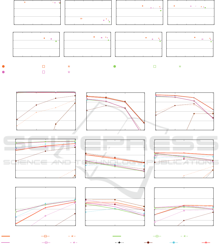
Figure 2 shows the average precision and recall

results for graphs with the lowest match threshold (θ)

for merge thresholds T in [0,1). The top row shows

the results for only clean sources, while the lower

row shows results for MSCD sources (mix of clean

and dirty camera sources). We compare the basic hi-

erarchical clustering schemes (S-Link, C-Link etc.)

Matching Entities from Multiple Sources with Hierarchical Agglomerative Clustering

Precision

Recall

0 0.2 0.4

0.6

0.8 1

0.4

0.6

0.8

DS-G, θ = 0.75

0 0.2 0.4

0.6

0.8 1

DS-M, θ = 0.35

0 0.2 0.4

0.6

0.8 1

DS-C100, θ = 0.30

0 0.2 0.4

0.6

0.8 1

DS-P2, θ = 0.60

0 0.2 0.4

0.6

0.8 1

0.4

0.6

0.8

DS-C0, θ = 0.30

0 0.2 0.4

0.6

0.8 1

DS-C26, θ = 0.30

0 0.2 0.4

0.6

0.8 1

DS-C50, θ = 0.30

0 0.2 0.4

0.6

0.8 1

DS-C80, θ = 0.30

0 0.2 0.4 0.6 0.8 1

0.4

0.6

0.8

Precision

MSCD S-LINK S-LINK

S-LINK w/o weak

MSCD C-LINK C-LINK

C-LINK w/o weak

MSCD A-LINK A-LINK

A-LINK w/o weak

Figure 2: Precision/recall for hierarchical clustering schemes.

0.75 0.80 0.85 0.90

0.8

0.85

0.9

0.95

DS-G

Precision

0.75 0.80 0.85 0.90

0.8

0.85

0.9

0.95

Recall

0.75 0.80 0.85 0.90

0.8

0.85

0.9

0.95

F-Measure

0.35 0.40 0.45

0.5

0.6

0.7

0.8

0.9

DS-M

0.35 0.40 0.45

0.5

0.6

0.7

0.8

0.9

0.35 0.40 0.45

0.5

0.6

0.7

0.8

0.9

0.60 0.70 0.80

0.7

0.8

0.9

DS-P2

0.60 0.70 0.80

0.7

0.8

0.9

0.60 0.70 0.80

0.7

0.8

0.9

0.30 0.50 0.70

0.6

0.7

0.8

0.9

DS-C100

MSCD S-LINK S-LINK

S-LINK w/o weak

MSCD C-LINK C-LINK

C-LINK w/o weak

MSCD A-LINK A-LINK

A-LINK w/o weak

ConCom CCPiv MSCD-AP CLIP

0.30 0.50 0.70

0.6

0.7

0.8

0.9

DS-C100

MSCD S-LINK S-LINK

S-LINK w/o weak

MSCD C-LINK C-LINK

C-LINK w/o weak

MSCD A-LINK A-LINK

A-LINK w/o weak

ConCom CCPiv MSCD-AP CLIP

Figure 3: Comparative evaluation of clustering schemes for MSC datasets.

with the ones applying the proposed MSCD exten-

sion. For all datasets except DC-C0 (with only dirty

sources), MSCD approaches improve precision dra-

matically while keeping the same recall; for DS-C0,

MSCD-HAC has the same results as the basic HAC.

Hence, the new MSCD approaches can clearly out-

perform the basic HAC schemes. Ignoring weak link

for the basic schemes can help improve precision in

several cases, but to a much smaller degree that with

MSCD. As expected, C-Link (S-LINK) achieves the

highest (lowest) precision and the lowest (highest) re-

call for all datasets due to the use of the minimal

(maximal) similarity between cluster members to de-

termine merge candidates. A-LINK follows a more

KEOD 2021 - 13th International Conference on Knowledge Engineering and Ontology Development

0.30 0.50 0.70

0.6

0.7

0.8

0.9

DS-C0

Precision

0.30 0.50 0.70

0.6

0.7

0.8

0.9

Recall

0.30 0.50 0.70

0.6

0.7

0.8

0.9

F-Measure

0.30 0.50 0.70

0.6

0.7

0.8

0.9

DS-C50

0.30 0.50 0.70

0.6

0.7

0.8

0.9

0.30 0.50 0.70

0.6

0.7

0.8

0.9

0.30 0.50 0.70

0.6

0.7

0.8

0.9

DS-C80

0.30 0.50 0.70

0.6

0.7

0.8

0.9

0.30 0.50 0.70

0.6

0.7

0.8

0.9

0.30 0.50 0.70

0.6

0.7

0.8

0.9

DS-C100

0.30 0.50 0.70

0.6

0.7

0.8

0.9

0.30 0.50 0.70

0.6

0.7

0.8

0.9

0.30 0.50 0.70

0.6

0.7

0.8

0.9

DS-C100

MSCD S-LINK S-LINK

S-LINK w/o weak

MSCD C-LINK C-LINK

C-LINK w/o weak

MSCD A-LINK A-LINK

A-LINK w/o weak

ConCom CCPiv MSCD-AP CLIP

0.30 0.50 0.70

0.6

0.7

0.8

0.9

DS-C100

MSCD S-LINK S-LINK

S-LINK w/o weak

MSCD C-LINK C-LINK

C-LINK w/o weak

MSCD A-LINK A-LINK

A-LINK w/o weak

ConCom CCPiv MSCD-AP CLIP

Figure 4: Comparative evaluation of clustering schemes for Camera datasets.

moderate strategy compared to the strict C-LINK and

relaxed S-LINK strategies. In addition, applying the

MSCD strategy or removing weak links improves S-

LINK the most, while C-LINK yields the same results

as basic HAC. Due to the fact that entities of the same

clean source are never directly linked to each other, C-

LINK obtains source-consistent clusters as the MSCD

approaches.

Figure 3 and Figure 4 show the results of our

proposed approaches for different match thresholds

θ and merge thresholds T (equal match and merge

threshold) for clean (MSC) and mixed (MSCD)

datasets in comparison with the baseline algorithm

connected components, Correlation clustering

(CCPivot variation) [Chierichetti et al., 2014] as

popular ER clustering schemes, the MSC algorithm

named CLIP [Saeedi et al., 2018] and the MSCD-AP

approach based on Afﬁnity Propagation [Lerm et al.,

2021]. We give a brief explanation of all mentioned

algorithms for a better understanding of the output

results.

Connected Components (ConCom): The sub-

graphs of a graph that are not connected to each other

are called connected components.

CCPivot (CCPiv): It is an estimation to the so-

lution of Correlation Clustering problem [Bansal

et al., 2002]. In each round of the algorithm, several

vertices are considered as active nodes (cluster center

or pivot). Then the adjacent vertices of each center

are assigned to that center and form a cluster. If

Matching Entities from Multiple Sources with Hierarchical Agglomerative Clustering

DS-G DS-M DS-C100 DS-P2

0,2

0,4

0,6

0,8

F-Measure

CLIP MSCD-AP MSCD S-LINK

DS-C0 DS-C26 DS-C50 DS-C80

0,2

0,4

0,6

0,8

F-Measure

CLIP MSCD-AP MSCD S-LINK

Figure 5: Average F-Measure results with range between minimal and maximal threshold values.

one vertex is adjacent of more than one center at

the same time, it will belong to the one with higher

priority. The vertex priorities are determined in a

preprocessing phase.

Multi-Source Clean Dirty Afﬁnity Propaga-

tion (MSCD-AP): The basic Afﬁnity Propagation

(AP) clusters entities by identifying exemplars

(cluster representative member or center). The goal

of AP is to ﬁnd exemplars and cluster assignments

such that the sum of inter-cluster similarities are max-

imized. MSCD-AP incorporates source-consistency

constraints into the basic AP.

CLIP: The algorithm classiﬁes the graph links

into three groups of Strong, Normal, and Weak by

considering all data sources as duplicate-free. It

then groups entities into source-consistent clusters

by omitting weak links in two phases. In phase one,

the strong links that form clusters with maximum

possible size (number of sources) are considered and

in phase two the remaining strong and normal links

are prioritized to form source-consistent clusters.

As expected for MSC datasets (Figure 3), con-

nected components and S-LINK obtain the lowest

precision. Removing weak links improves precision

for S-LINK, but it is still not sufﬁcient to compete

with the best algorithms. The C-LINK approaches

and MSCD-AP achieve the best precision, but at the

cost of low recall. In contrast, CLIP and MSCD

S-LINK obtain similarly high recall and precision.

Therefore, for all datasets, MSCD S-LINK and CLIP

are superior in terms of F-Measure and outperform

the basic HAC approaches as well as the previous

MSCD-AP approach for mixed datasets. For the big-

ger dataset DS-P, CLIP and MSCD S-LINK obtain

lower precision compared to MSCD A-LINK, be-

cause they form clusters with the maximum possible

size (10, one entity per source) which leads to obtain-

ing false positives. Therefore, MSCD A-LINK sur-

passes MSCD S-LINK and CLIP for the low thresh-

old 0.6.

For MSCD datasets (Figure 4), MSCD-HAC and

HAC give the same results for the dataset with all

dirty sources (DS-C0). Therefore, for DS-C0, MSCD

S-LINK along with connected components obtains

the lowest precision and the highest recall. As the

ratio of clean sources increases, MSCD S-LINK ob-

tains better precision while keeping the recall high.

Therefore, for all MSCD datasets, MSCD S-LINK

obtains the best F-Measure. The algorithm CLIP

yields very low F-Measure, because it is designed for

clustering clean datasets. The algorithm MSCD-AP

can not compete with MSCD-HAC approaches due

to its lower recall (about 10% less than MSCD S-

LINK). When the dataset comprises a large portion

of or only dirty sources, the strict method MSCD C-

LINK obtains the best results for lower thresholds. In

all datasets except for DS-C0, CCPiv can not com-

pete with the best algorithms in both terms of preci-

sion and recall. With DS-C0, CCPiv is slightly better

than A-LINK due to the higher recall it achieves. Due

to space restrictions, we omitted results for DS-P1 and

some MSCD datasets, but they follow the same trends

as discussed.

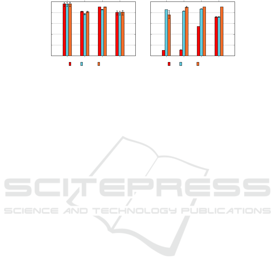
Figure 5 conﬁrms the results shown in Figure 3

and Figure 4. It shows the average F-Measure results

of the CLIP (MSC clustering scheme), MSCD-AP,

and S-LINK over all matching threshold (θ) conﬁg-

urations. As depicted in Figure 5, for clean datasets

(left ﬁgure) MSCD-HAC with S-LINK strategy com-

petes with CLIP, while for the dirty datasets (right ﬁg-

ure), it is superior (except for DS-C0 which does not

contain any clean source) compared to both CLIP and

MSCD-AP clustering schemes. Moreover, the aver-

age F-Measure of S-LINK shows robustness against

the degree of dirtiness.

5.3 Runtimes and Speedup

We evaluate runtimes and speedup behavior for the

larger datasets from the person domain for the graph

with match and merge threshold θ = T = 0.8. The

experiments are performed on a shared nothing clus-

KEOD 2021 - 13th International Conference on Knowledge Engineering and Ontology Development

ter with 16 worker nodes. Each worker consists of

an E5-2430 6(12) 2.5 Ghz CPU, 48 GB RAM, two 4

TB SATA disks and runs openSUSE 13.2. The nodes

are connected via 1 Gigabit Ethernet. Our evaluation

is based on Hadoop 2.6.0 and Flink 1.9.0. We run

Apache Flink standalone with 6 threads and 40 GB

memory per worker. Table 6 lists runtimes of all intro-

duced approaches evaluated on 16 machines. The ﬁrst

row shows that S-LINK is the slowest algorithm, but

MSCD S-LINK improves the runtime of S-LINK dra-

matically. Moreover, removing weak links decreases

runtime slightly. Neither applying MSCD strategy

nor removing weak links improves the runtime of C-

LINK and A-LINK, because the approaches are strict

enough in merging clusters. The last four rows of

Table 6 list the runtime of approaches that are com-

pared with HAC-based schemes. Among them, con-

nected components is the fastest approach while CLIP

and MSCD-AP are 1.4x-2x faster and CCPiv is 2x-

3.5x slower than HAC-based approaches. Figure 6

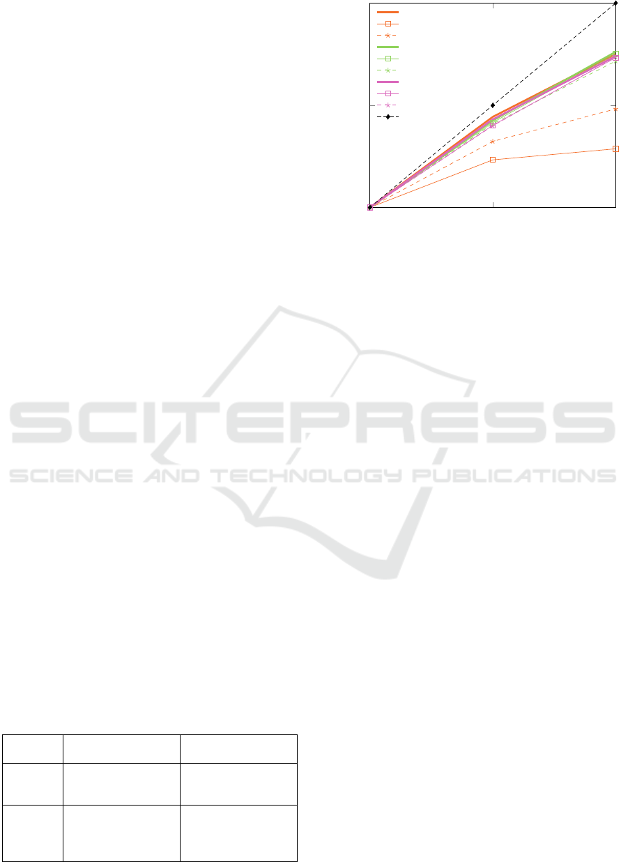
shows the speedup for DS-P1 with 5M entities. All

approaches have speedup close to linear, expect S-

LINK. Removing weak links improves the speedup

of S-LINK, but it is still far from linear speedup. The

approaches can not utilize 16 machines so that a good

speedup is achieved until 8 workers.

6 CONCLUSION AND OUTLOOK

We proposed an extension of hierarchical agglomera-

tive clustering called MSCD-HAC to perform multi-

source entity clustering for a mix of clean and dirty

data sources. The evaluation of MSCD-HAC with

different linkage types showed that MSCD S-LINK

obtains superior cluster results compared to previous

clustering schemes speciﬁcally for MSCD datasets

with dirty sources. For the case of clean sources the

same or better quality than the best methods such as

CLIP is achieved. In some cases such as for larger

clusters (many sources), MSCD S-LINK is outper-

formed by other linkage strategies. We will therefore

investigate how to automatically select the best link-

age strategy for MSCD clustering.

Table 6: Runtimes (second).

DS-P1 DS-P2

- MSCD NW - MSCD NW

S-LINK 2256 130 2149 6818 506 6789

C-LINK 128 128 130 422 417 401

A-LINK 127 129 128 430 417 411

ConCom 37 59

CCPiv 463 1030

MSCD-AP 93 207

CLIP 80 200

4 8 16

No. of Machines

Speedup

MSCD S-LINK

S-LINK

S-LINK w/o weak

MSCD C-LINK

C-LINK

C-LINK w/o weak

MSCD A-LINK

A-LINK

A-LINK w/o weak

Linear

Figure 6: Speedup.

ACKNOWLEDGEMENTS

This work is partially funded by the German

Federal Ministry of Education and Research un-

der grant BMBF 01IS18026B in project ScaDS.AI

Dresden/Leipzig.

REFERENCES

Bansal, N., Blum, A., and Chawla, S. (2002). Correla-

tion clustering. In 43rd Symposium on Foundations

of Computer Science (FOCS 2002), 16-19 Novem-

ber 2002, Vancouver, BC, Canada, Proceedings, page

238. IEEE Computer Society.

Chierichetti, F., Dalvi, N. N., and Kumar, R. (2014). Corre-

lation clustering in mapreduce. In Macskassy, S. A.,

Perlich, C., Leskovec, J., Wang, W., and Ghani, R.,

editors, The 20th ACM SIGKDD International Con-

ference on Knowledge Discovery and Data Mining,

KDD ’14, New York, NY, USA - August 24 - 27, 2014,

pages 641–650. ACM.

Dahlhaus, E. (2000). Parallel algorithms for hierarchical

clustering and applications to split decomposition and

parity graph recognition. J. Algorithms, 36(2):205–

240.

Dash, M., Petrutiu, S., and Scheuermann, P. (2007). ppop:

Fast yet accurate parallel hierarchical clustering using

partitioning. Data Knowl. Eng., 61(3):563–578.

Hassanzadeh, O., Chiang, F., Miller, R. J., and Lee, H. C.

(2009). Framework for evaluating clustering algo-

rithms in duplicate detection. Proc. VLDB Endow.,

2(1):1282–1293.

Hendrix, W., Patwary, M. M. A., Agrawal, A., Liao, W.,

and Choudhary, A. N. (2012). Parallel hierarchical

clustering on shared memory platforms. In 19th Inter-

national Conference on High Performance Comput-

Matching Entities from Multiple Sources with Hierarchical Agglomerative Clustering

ing, HiPC 2012, Pune, India, December 18-22, 2012,

pages 1–9. IEEE Computer Society.

Jin, C., Liu, R., Chen, Z., Hendrix, W., Agrawal, A., and

Choudhary, A. N. (2015). A scalable hierarchical

clustering algorithm using spark. In First IEEE In-

ternational Conference on Big Data Computing Ser-

vice and Applications, BigDataService 2015, Red-

wood City, CA, USA, March 30 - April 2, 2015, pages

418–426. IEEE Computer Society.

Junghanns, M., Petermann, A., Neumann, M., and Rahm, E.

(2017). Management and analysis of big graph data:

Current systems and open challenges. In Zomaya,

A. Y. and Sakr, S., editors, Handbook of Big Data

Technologies, pages 457–505. Springer.

Kaufman, L. and Rousseeuw, P. J. (1990). Finding Groups

in Data: An Introduction to Cluster Analysis. John

Wiley.

Koga, H., Ishibashi, T., and Watanabe, T. (2007). Fast

agglomerative hierarchical clustering algorithm using

locality-sensitive hashing. Knowl. Inf. Syst., 12(1):25–

53.

Lerm, S., Saeedi, A., and Rahm, E. (2021). Extended afﬁn-

ity propagation clustering for multi-source entity res-

olution. In Sattler, K., Herschel, M., and Lehner,

W., editors, Datenbanksysteme f

ur Business, Tech-

nologie und Web (BTW 2021), 19. Fachtagung des

GI-Fachbereichs ,,Datenbanken und Informationssys-

teme” (DBIS), 13.-17. September 2021, Dresden, Ger-

many, Proceedings, volume P-311 of LNI, pages 217–

236. Gesellschaft f

ur Informatik, Bonn.

Mamun, A.-A., Aseltine, R., and Rajasekaran, S. (2016).

Efﬁcient record linkage algorithms using complete

linkage clustering. PloS one, 11(4):e0154446.

Murtagh, F. (1983). A survey of recent advances in hierar-

chical clustering algorithms. Comput. J., 26(4):354–

359.

Murtagh, F. and Contreras, P. (2012). Algorithms for hierar-

chical clustering: an overview. Wiley Interdiscip. Rev.

Data Min. Knowl. Discov., 2(1):86–97.

Nentwig, M., Groß, A., and Rahm, E. (2016). Holis-

tic entity clustering for linked data. In Domeni-

coni, C., Gullo, F., Bonchi, F., Domingo-Ferrer,

J., Baeza-Yates, R., Zhou, Z., and Wu, X., edi-

tors, IEEE International Conference on Data Mining

Workshops, ICDM Workshops 2016, December 12-15,

2016, Barcelona, Spain, pages 194–201. IEEE Com-

puter Society.

Nielsen, F. (2016). Introduction to HPC with MPI for Data

Science. Undergraduate Topics in Computer Science.

Springer.

Rokach, L. and Maimon, O. (2005). Clustering methods. In

Maimon, O. and Rokach, L., editors, The Data Mining

and Knowledge Discovery Handbook, pages 321–352.

Springer.

Saeedi, A., Peukert, E., and Rahm, E. (2017). Com-

parative evaluation of distributed clustering schemes

for multi-source entity resolution. In Kirikova, M.,

Nørv

ag, K., and Papadopoulos, G. A., editors, Ad-

vances in Databases and Information Systems - 21st

European Conference, ADBIS 2017, Nicosia, Cyprus,

September 24-27, 2017, Proceedings, volume 10509

of Lecture Notes in Computer Science, pages 278–

293. Springer.

Saeedi, A., Peukert, E., and Rahm, E. (2018). Using link

features for entity clustering in knowledge graphs.

In Gangemi, A., Navigli, R., Vidal, M., Hitzler, P.,

Troncy, R., Hollink, L., Tordai, A., and Alam, M., ed-

itors, The Semantic Web - 15th International Confer-

ence, ESWC 2018, Heraklion, Crete, Greece, June 3-

7, 2018, Proceedings, volume 10843 of Lecture Notes

in Computer Science, pages 576–592. Springer.

Ward Jr, J. H. (1963). Hierarchical grouping to optimize an

objective function. Journal of the American statistical

association, 58(301):236–244.

Yan, Y., Meyles, S., Haghighi, A., and Suciu, D. (2020).

Entity matching in the wild: A consistent and ver-

satile framework to unify data in industrial applica-

tions. In Maier, D., Pottinger, R., Doan, A., Tan, W.,

Alawini, A., and Ngo, H. Q., editors, Proceedings of

the 2020 International Conference on Management of

Data, SIGMOD Conference 2020, online conference

[Portland, OR, USA], June 14-19, 2020 , pages 2287–

2301. ACM.

KEOD 2021 - 13th International Conference on Knowledge Engineering and Ontology Development