A Hybrid Evolutionary Algorithm, Utilizing Novelty Search and Local

Optimization, Used to Design Convolutional Neural Networks for

Handwritten Digit Recognition

Tabish Ashfaq, Nivedha Ramesh and Nawwaf Kharma

Department of Electrical and Computer Engineering, Concordia University, Montreal, Quebec, Canada

Keywords:

Neuroevolution, Evolutionary Algorithms, Convolutional Neural Networks, Deep Learning, Cartesian

Genetic Programming, Genetic Algorithms, Stochastic Local Search, Novelty Search, Simulated Annealing.

Abstract:

Convolutional neural networks (CNNs) are deep learning models that have been successfully applied to vari-

ous computer vision tasks. The design of CNN topologies often requires extensive domain knowledge and a

high degree of trial and error. In recent years, numerous Evolutionary Algorithms (EAs) have been proposed to

automate the design of CNNs. The search space of these EAs is very large and often deceptive, which entails

great computational cost. In this work, we investigate the design of CNNs using Cartesian Genetic Program-

ming (CGP), an EA variant. We then augment the basic CGP with methods for identifying potential/actual

local optima within the solution space (via Novelty Search), followed by further local optimization of each of

the optima (via Simulated Annealing). This hybrid EA methodology is evaluated using the MNIST data-set

for handwritten digit recognition. We demonstrate that the use of the proposed method results in considerable

reduction of computational effort, when compared to the basic CGP approach, while still returning competitive

results. Also, the CNNs designed by our method achieve competitive recognition results compared to other

neuroevolutionary methods.

1 INTRODUCTION

Image recognition is a widely studied application of

computer vision. In recent years Convolutional Neu-

ral Networks (CNNs) have proven to be especially ef-

fective at this task in a supervised learning context.

This has motivated the development of numerous evo-

lutionary algorithms (EAs) for the design of CNN ar-

chitectures and for the optimization of their hyperpa-

rameters (Baldominos et al., 2018; Xie and Yuille,

2017; McGhie et al., 2020).

The computational effort expended by such algo-

rithms in obtaining optimal solutions is considerable,

and thus, such an approach may not be a viable op-

tion when computational resources are constrained.

As with many applications of evolutionary comput-

ing, a large proportion of the computational effort is

expended in evaluating a population of individual so-

lutions, many of which may be highly unﬁt or simply

redundant. As such, if a candidate solution is deter-

mined (by some criteria) to be useless, it may be re-

moved from the population, which saves on compu-

tational time without degrading the effectiveness of

evolutionary search and optimization.

Therefore, we are motivated to investigate modi-

ﬁcations to the standard evolutionary approach which

may lead to a more efﬁcient neural architecture search

procedure. This implies that potential solutions to the

problem should aim to reduce the number of wasted

cycles in the evolution process. This may be done

by identifying local optima within the solution space

and restricting the search to the neighbourhoods of

these local optima. For this purpose, we present a

method for approximate quantiﬁcation of structural

diversity and for characterization of local neighbour-

hoods within a population of CNNs.

In this work, we investigate the use of a three-

stage evolutionary optimization approach. The ﬁrst

stage in this approach aims to generate a diverse ini-

tial generation of CNNs using the Novelty Search al-

gorithm (Lehman and Stanley, 2011). The second

stage involves the evolution of CNN architectures us-

ing Cartesian Genetic Programming (CGP) (Miller

and Thomson, 2000). In the third stage, we select

the most diverse generation from the previous stage.

From this population, we sample the most optimal in-

dividuals in terms of both ﬁtness and novelty, using

a multi-objective optimization algorithm. We attempt

Ashfaq, T., Ramesh, N. and Kharma, N.

A Hybrid Evolutionary Algorithm, Utilizing Novelty Search and Local Optimization, Used to Design Convolutional Neural Networks for Handwritten Digit Recognition.

DOI: 10.5220/0010648300003063

In Proceedings of the 13th International Joint Conference on Computational Intelligence (IJCCI 2021), pages 123-133

ISBN: 978-989-758-534-0; ISSN: 2184-3236

123

to exploit the local neighbourhoods of these individ-

uals using a stochastic local search (SLS) algorithm.

The SLS algorithm implemented for this paper is the

Simulated Annealing (SA) (Kirkpatrick et al., 1983)

algorithm.

The rest of this paper is organised as follows.

Section 2 provides a review of related work in neu-

roevolution. Section 3 describes the genetic encoding,

and our optimized evolutionary approach to design-

ing CNN architectures. We present the results of our

proposed methodology in Section 4. Finally, we end

with some concluding remarks and recommendations

for future work in Section 5.

2 RELATED WORK

Neuroevolution has been used to design various types

of neural network weights and topologies to address

a wide range of problems. In 2002, the highly

inﬂuential technique, Neuroevolution of Augment-

ing Topologies (NEAT) (Stanley and Miikkulainen,

2002), was developed and proved effective in evolv-

ing the architecture and weights of small neural net-

works. In 2009, this method was extended with the

introduction of the HyperNEAT algorithm (Stanley

et al., 2009), which allowed for the evolution of larger

scale neural networks through indirect encoding using

a Compositional Pattern Producing Network (CPNN).

However, this technique has been shown to be inef-

fective in performing image classiﬁcation, and has re-

sulted in an error rate of 7.9% on the MNIST dataset

when used for feature learning with a CNN (Verbanc-

sics and Harguess, 2015).

In recent years, several works have been pub-

lished which attempt to automate the design of CNNs

through neuroevolution. Genetic CNN (Xie and

Yuille, 2017) is a Genetic Algorithm which uses a

ﬁxed-length binary string representation. The au-

thors obtained competitive recognition results on the

MNIST dataset. However, they do not encode the

fully-connected part of the network, choosing to adapt

the fully-connected part of the basic LeNet architec-

ture (Lecun et al., 1998).

Baldominos et al. (Baldominos et al., 2018) stud-

ied the evolution of CNNs using both a GA with bi-

nary Gray encoding representation, as well as Gram-

matical Evolution which uses an integer-based en-

coding. They include both convolutional and fully-

connected components in their frameworks, in addi-

tion to parameterizing the connectivity pattern within

the networks, thereby allowing for the evolution of

recurrent structures. The authors also present a sim-

ilarity metric which they use to implement a niching

strategy. However, the metric presented in this paper

evaluates to zero for individuals with unequal num-

bers of convolutional and dense layers, and hence,

it does not provide a measure of similarity in many

cases.

Sun et al. (Sun et al., 2020) propose a GA

which encodes highly functional blocks in variable-

length chromosomes, and incorporates skip connec-

tions. Similarly, a CGP-based approach (Suganuma

et al., 2017) was published in 2017 which uses a func-

tion set of convolutional and residual units to reduce

the search space. In both of these cases, only the con-

volutional part of the network is encoded. In addi-

tion, these works do not attempt to measure structural

similarity between different neural networks. In this

work, we augment the CGP approach introduced by

Suganuma et al. by extending the function set and

incorporating transpose convolutions and fully con-

nected layers.

3 METHODS

We evolve two separate populations of CNNs. The

ﬁrst of these populations, is optimized according to

the ﬁtness criteria described in Section 3.2.2, begin-

ning with a randomly generated initial generation.

This population is henceforth referred to as Popula-

tion 1. In the second population, Population 2, as an

alternative to random initialization, we include a dis-

tinct initialization stage. In this stage, we begin with

a randomly generated population and optimize it for

novelty, using the Novelty Search algorithm (Lehman

and Stanley, 2011) along with the metric developed

in Section 3.3. This process yields the initial genera-

tion for the evolutionary algorithm. Lastly, we apply

a different survivor selection scheme during evolution

of each of the two populations, as described in Section

3.2.3.

The individual networks evolved in our algorithms

are each designed as a combination of two sub-

networks: a fully convolutional network followed by

a fully connected (dense) network.

3.1 Genetic Encoding

For the encoding of the fully convolutional sub-

network, we adapt a CGP based approach (Suganuma

et al., 2017) which uses the functional modules de-

scribed in Table 1 as the node functions. The fully-

connected sub-network is represented using a list of

node functions drawn from a function set of dense

layers. Thus, the genotype may be considered as the

combination of a CGP grid - where each element of

ECTA 2021 - 13th International Conference on Evolutionary Computation Theory and Applications

124

the grid contains a function gene as well as a connec-

tion gene - and a list of fully-connected node func-

tions.

The combination of these two encodings is ex-

pressed as a directed acyclic graph (DAG). The DAG

is an intermediate phenotype which may be adjusted

to ensure the validity of networks generated for a

given classiﬁcation task. For the MNIST dataset, we

enforce the output layer of each network to be a dense

layer with 10 nodes and a softmax activation function.

Finally, the DAG representation is used to con-

struct the CNN, which is implemented as a Keras

(Chollet et al., 2015) model. In the remainder of this

paper, the CNN is referred to as the phenotype.

3.1.1 Representation of the Fully Convolutional

Sub-network

The fully-convolutional sub-network is represented

using a two-dimensional matrix, in which each ele-

ment of the matrix contains a string that describes the

node function gene as well as the indices of the input

nodes. Seven types of node functions are prepared

and included in the function set, namely, ConvBlock,

ResBlock, DeconvBlock, max pooling, average pool-

ing, concatenation, and summation.

The ConvBlock consists of standard convolution

processing with a stride of 1, followed by batch nor-

malization and a ReLU activation function. All con-

volutions are same convolutions, i.e. the input to the

convolution operation is padded with zeros, result-

ing in an output that matches the input in terms of

height and width of the activation map. Thus, the

height and width of an activation map is reduced only

through pooling layers. The function set contains

ConvBlocks of different numbers of output channels

and kernel sizes. ResBlocks are composed of Con-

vBlocks followed by a second convolution operation,

batch normalization, summation, and ﬁnally ReLU

activation. DeconvBlocks consists of a convolution

operation followed by batch normalization, ReLU ac-

tivation, and ﬁnally upsampling by a factor of 2.

The max pooling and average pooling functions

are applied over a window size of 2, using a stride

value of 2. The concatenation function takes two ac-

tivation maps as input, and concatenates them along

the feature axis. In the case where the two activa-

tion maps have unequal height and width, the larger

activation map is downsampled by max pooling prior

to concatenation. Finally, the summation function is

used to add the values of two activation maps. In cases

where direct summation is not possible due to incom-

patible numbers of channels in the activation maps,

the number of channels in the smaller of the two acti-

vation maps is increased by applying 1-by-1 convolu-

tion prior to summation.

3.1.2 Representation of the Fully-connected

Sub-network

The fully-connected sub-network is represented as a

list of DenseBlock node functions as described in Ta-

ble 1. This network is then appended to the output of

the fully convolutional sub-network. As mentioned

above, a softmax output layer with 10 nodes is ap-

pended to the end of the fully-connected network.

Figure 1 illustrates the genotype of the ﬁttest solution

obtained by the proposed method.

3.2 Evolutionary Algorithm

Evolutionary strategies belong to the family of evo-

lutionary algorithms and are majorly applied to opti-

mization problems. The search paradigm inspired by

biological evolution involves applying mutation, re-

combination and selection operators to a population

of candidate solutions. In our work, we adopt the (20

+ λ) evolutionary strategy to evolve CNN architec-

tures. We use a value of λ = 16. An initial population

of 20 individuals is randomly generated subject to ini-

tialization constraints which ensure that the resulting

CNNs will ﬁt in the available GPU memory.

3.2.1 Mutation Operators

Variation in the population is introduced through mu-

tation of function and connection genes – that is, a

given node may have its function swapped with a ran-

dom selection from the function set, or may have its

immediate neighbours swapped.

3.2.2 Fitness Evaluation

Each individual is trained on the MNIST training set

for 5 epochs, after which it is evaluated on the held-

out validation set. It should be noted that the test set

is not used for evaluation during evolution. Training

hyperparameters are kept constant for all individuals.

We use the Adam optimization algorithm (Kingma

and Ba, 2017) to minimize Categorical Cross-Entropy

loss. A learning rate of 1e-4 is used during training for

all individuals.

The partially trained networks are then evaluated

using the F

score, deﬁned in (1), where TP: true pos-

itive, FP: false positive, FN: false negative:

T P

(T P +

(FP + FN))

(1)

A Hybrid Evolutionary Algorithm, Utilizing Novelty Search and Local Optimization, Used to Design Convolutional Neural Networks for

Handwritten Digit Recognition

125

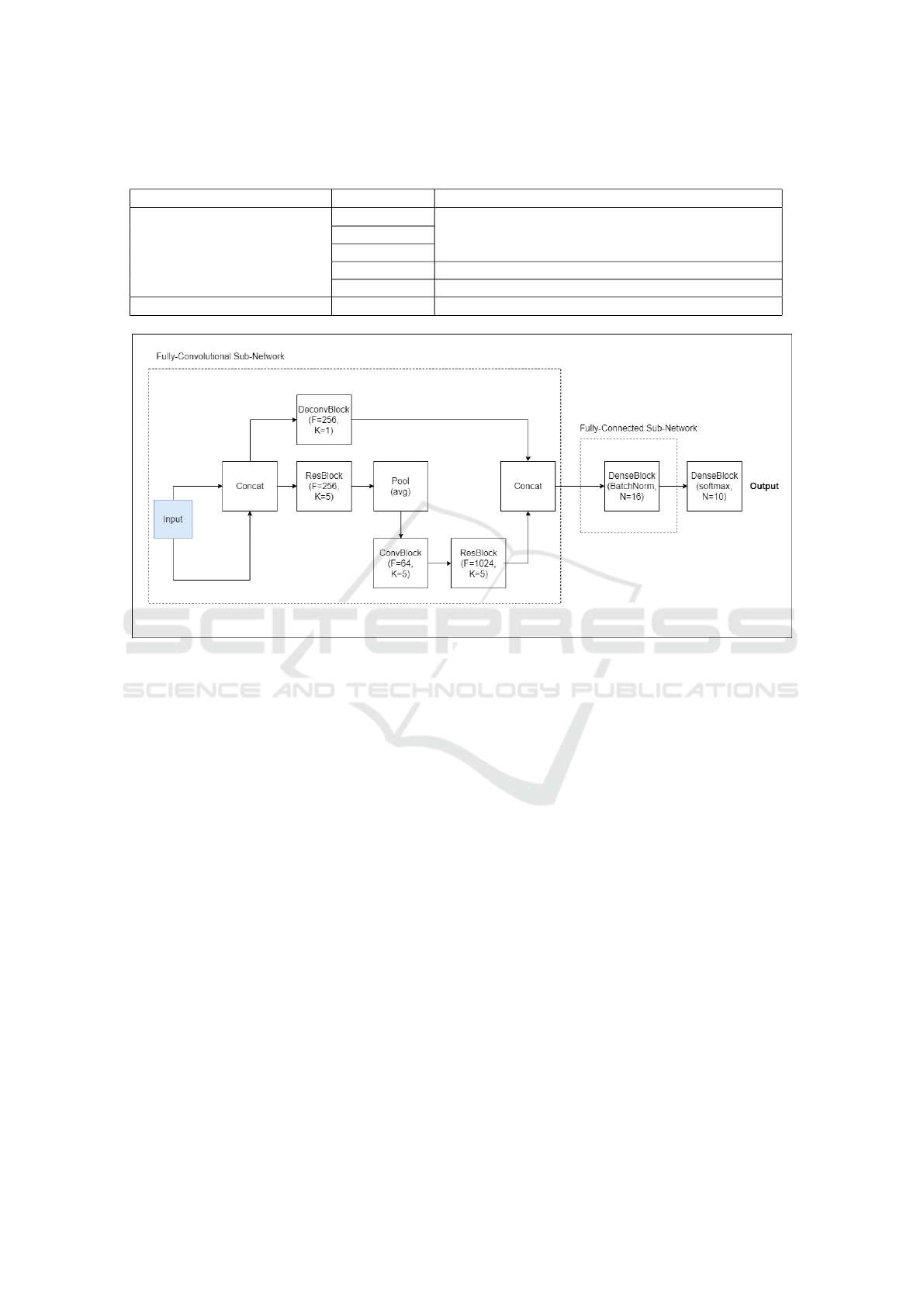
Table 1: Node functions present in the CGP function set. F: number of ﬁlters (output channels), K: kernel size, N: number

of units in a dense layer.

Sub-Network Node Type Variation

Fully-Convolutional Network

ConvBlock

F = {1, 2, 4, 8, 16, 32, 64, 128, 256, 512, 1024}

K = {1, 3, 5}

ResBlock

DeconvBlock

Pooling Average pooling, Max pooling

MergeBlock Summation, Concatenation

Fully-Connected Network DenseBlock N = {8, 16, 32, 64, 128, 256, 512, 1024, 2048, 4096}

Figure 1: Genotype of the best performing CNN architecture obtained by the proposed method. The ﬁgure demonstrates how

the active path of the CGP genotype is expressed, resulting in an encoding that describes the CNN in terms of the highly

functional modules enumerate in Table 1.

3.2.3 Parent Selection and Survivor Selection

For parent selection, we use tournament selection

(Miller and Goldberg, 1995) from the current gen-

eration with a window size of 5. We select 20% of

the population without replacement. For survivor se-

lection, we use tournament selection from the pool

of parents and offspring of the current generation,

without replacement. A window size of 5 is used.

We favour individuals with smaller model size, where

model size is deﬁned as the number of trainable pa-

rameters of a CNN. Thus, when comparing two indi-

viduals, the lesser ﬁt of the two may be selected if: (1)

its ﬁtness lies within a tolerance of 0.05 of the ﬁtter

individual, and (2) it has fewer trainable parameters

than the ﬁtter individual. In the case of the second

population, survivor selection is realised in a similar

manner: the ﬁrst clause is the same as above. The

second clause is amended to favour individuals with a

higher novelty score: the lesser ﬁt of two individuals

may be selected if it has fewer trainable parameters,

or has a higher novelty score, than the ﬁtter individ-

ual.

3.2.4 Offspring Generation

Offspring are generated from parents using the afore-

mentioned mutation operators. In the case that a child

is produced via a mutation that does not alter the ac-

tive path (the longest list of connected nodes) its ﬁt-

ness is set equal to that of its parent.

3.2.5 Termination Criteria

Evolution is terminated after 200 generations, result-

ing in 3204 ﬁtness evaluations.

3.3 Diversity Measures and Novelty

In order to study the effect of structural diversity on

the efﬁciency of the evolutionary algorithm in obtain-

ing optimal solutions, a second population is gen-

erated using the Novelty Search algorithm (Lehman

and Stanley, 2011). The resulting population is then

used as the initial population for the evolutionary al-

gorithm, following the procedure described in the pre-

ECTA 2021 - 13th International Conference on Evolutionary Computation Theory and Applications

126

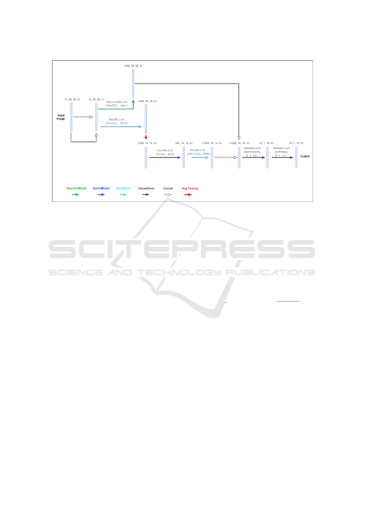
Figure 2: Phenotype of the best performing CNN architecture obtained by the proposed method, with the vector representation

of each layer indicated. The ﬁgure illustrates the functions of each of the modules represented in the genotype illustrated in

Figure 1. The coloured arrows indicate the various functions: DeconvBlock (green), ConvBlock (blue), ResBlock (cyan),

DenseBlock (dark gray), Concatenation (white), and Average Pooling (red).

vious section. This is the aforementioned Population

We develop a novelty metric based on cosine

similarity as deﬁned below. This metric is used in

our Novelty Search algorithm to explore the solution

space.

3.3.1 Vector Representation of the CNN

The structural information in the phenotype of can-

didate solutions is represented using sets of 4-

dimensional vectors, where each vector represents a

successive layer of the CNN. This is illustrated in Fig-

ure 2. A single layer, v

, in a CNN architecture can

be represented as in (2).













(2)

Where c

, x

and y

describe the size of the layer’s

activation in terms of the numbers of channels, the

width, and the height, respectively. The parameter d

represents the depth of the layer, i.e., the minimum

number of layers between this layer and the input

layer.

This representation allows us to obtain an approx-

imate measure of the structural similarity between so-

lutions using vector similarity measures such as co-

sine similarity.

3.3.2 Cosine Similarity and K Nearest

Neighbours Computation

The cosine similarity between two vectors is deﬁned

as in (3).

cosine similarity(v

) =

· v

(|v

||v

(3)

The similarity between two individuals is com-

puted as described by Algorithm 1. The novelty of

an individual is then calculated using the normalized

sum of its similarity with its k nearest neighbours

(Cover and Hart, 1967), with k=11. This value is then

scaled by a factor of 100, and the result is subtracted

from 100. Thus, novelty scores lie within the range of

0-100.

3.4 Local Optimization

The proposed method involves the use of EAs for ex-

ploration and the use of an SLS algorithm for the local

optimization of near-optima. In order to demonstrate

this procedure, we select from Populations 1 and 2 the

generations with highest mean novelty, as illustrated

in Figure 3. The novelty score of an individual is as

deﬁned in Section 3.3.2. Thus, every architecture in

A Hybrid Evolutionary Algorithm, Utilizing Novelty Search and Local Optimization, Used to Design Convolutional Neural Networks for

Handwritten Digit Recognition

127

Algorithm 1: Computing similarity between two individu-

als.

Result: norm sum

V1: vector set representation of individual 1

V2: vector set representation of individual 2

similarity: array of length max(length(V1),

length(V2))

norm sum: normalized element-wise sum of

similarity array

V1 = V1[1:length(V1)-1];

V2 = V2[1:length(V2)-1];

if length(V2) >length(V1) then

temp ← V 1;

V 1 ← V2;

V 2 ← temp;

end

for i ← 0 to length(V1) - length(V2) do

V2.append([0,0,0,0])

end

for i ← 0 to length(V1) do

if norm(V2) = 0 then

similarity[i] ← 0;

else

similarity[i] ←

cosine similarity(V 1[i],V 2[i]);

end

norm sum ←

sum(similarity)/length(similarity)

each of these sampled generations contains an evalu-

ation score (F

Score) and a novelty score. Based on

these two metrics, we select individuals which are de-

termined to be located near/at local optima. We then

perform an extensive search of their local neighbor-

hood to discover optimal architectures.

Here, we distinguish two other populations: the

group of individuals selected for local optimization

from Population 1 is henceforth referred to as Popu-

lation 3. Similarly, the group of individuals selected

from Population 2 will be referred to as Population 4.

3.4.1 Identiﬁcation of Local Optima

As every architecture has an evaluation metric and

a novelty metric, the sampling of local optima can

be treated as a multi-objective optimization problem.

Among the many existing evolutionary algorithms for

multi-objective optimization, we use the NSGA-II al-

gorithm. NSGA-II has evolved over the last few years

with many new variants (D’Souza et al., 2010) which

have reduced its time-complexity or/and improved its

convergence to the true Pareto Optimal front.

The algorithm proceeds by performing a non-

dominated sorting of the CNN structures based on

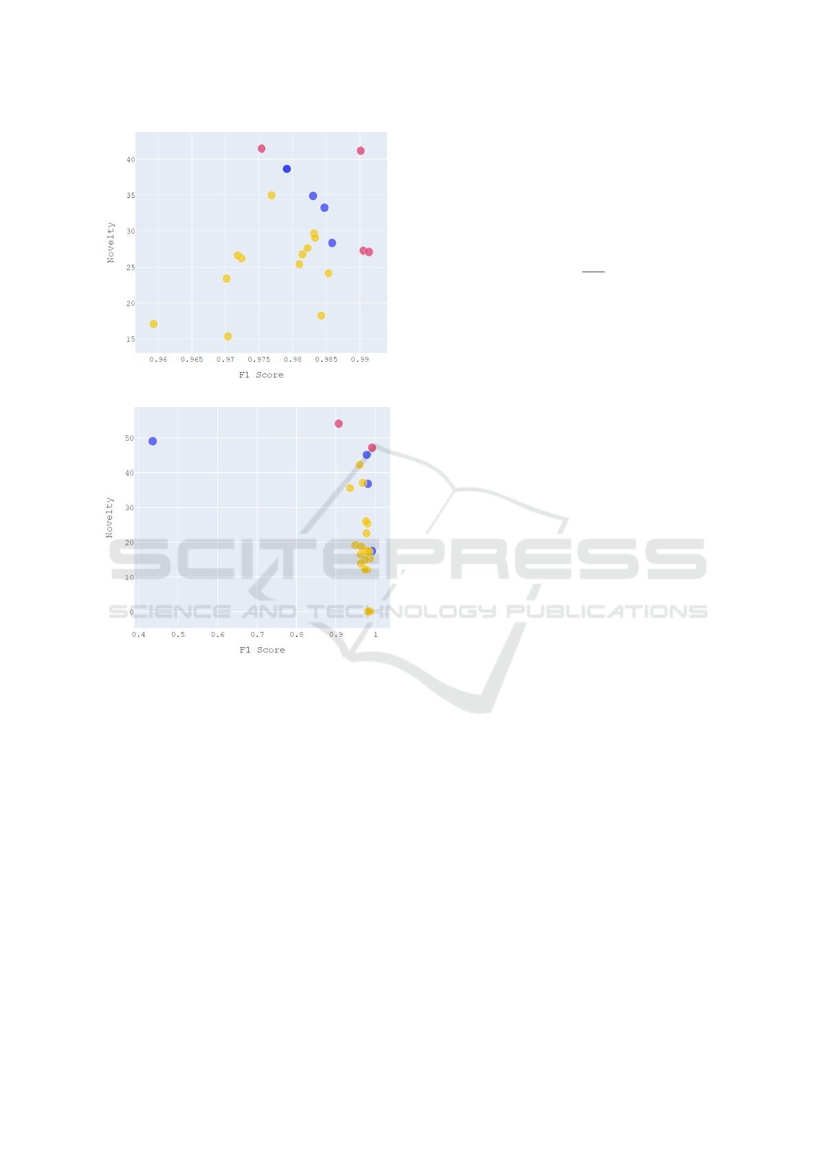
(a) Variation of mean novelty over different generations of

the evolutionary algorithm for Population 1.

(b) Variation of mean novelty over different generations of

the evolutionary algorithm for Population 2, which is

optimized for ﬁtness and novelty.

Figure 3: Mean novelty vs time: evolutionary algorithm

(top) and evolutionary algorithm with Novelty Search (bot-

tom). In each case, the vertical line indicates the generation

selected for local optimization.

their multi-objective ﬁtness values, and ranking the

solutions into different non dominated fronts as in

Figure 4. Thereafter, we sample the solutions by

selecting those individuals belonging to the highest

ranked front ﬁrst, followed by those of the next front

and so on, until we have obtained at least 4 individ-

uals. In case there is space only for part of a front

in the new population, we use a crowded-distance op-

erator to determine the individuals that are from the

least crowded regions within that front. Details of the

crowded-distance operator can be obtained from (Deb

et al., 2002).

The solutions sampled from Population 1 comprise

rank 1 and rank 2 solutions, while the four solutions

sampled from Population 2 comprise rank 1 solutions

only. These constitute the Population 3 and 4, respec-

tively.

ECTA 2021 - 13th International Conference on Evolutionary Computation Theory and Applications

128

(a) Pareto Optimal Front for Population 1.

(b) Pareto Optimal Fronts for Population 2.

Figure 4: The generation with the highest mean novelty

score that is sampled from Population 1 and Population 2

is fed into the NSGA II algorithm. The solutions in pink

belong to rank 1, solutions in blue belong to rank 2 and so-

lutions in yellow belong to further lower ranks.

3.4.2 Simulated Annealing

The solutions found by NSGA II are fed into a local

search optimizer. A local search algorithm explores

the neighborhood of a candidate by comparing it with

neighboring solutions. This search is guided by a cost

function that measures the quality of a given solution.

In our work, we have chosen Simulated Annealing

as the local optimization algorithm. Simulated An-

nealing is a heuristic method which was inspired by

the physical annealing of metals (Kirkpatrick et al.,

1983). The search algorithm iteratively compares a

given solution to another neighboring solution in the

local neighborhood of the current solution. The cost

function reﬂects the difference between the ﬁtness of

the current solutions and that of a neighbour. If the

cost is positive (neighbour is ﬁtter), the algorithm se-

lects the neighboring solution as the (working) opti-

mal one for the next iteration. However, if the cost

is negative, the algorithm selects either solution (cur-

rent or neighbour), on a probabilistic basis described

by (4).

P = exp(

cost

) (4)

The algorithm starts with an initial ’high temper-

ature’, when the probability of accepting bad solu-

tions is higher. This ensures that the algorithm does

not get stuck in a local optimum. The temperature

is iteratively reduced in line with a cooling schedule.

The most popular cooling schedule is the geometric

cooling schedule, which deﬁnes a parameter α with

a value between 0 and 1. At the conclusion of every

iteration, the temperature is updated in line with (5).

T = α ∗ T (5)

As the algorithm progresses the temperature de-

creases exponentially according to the cooling sched-

ule, making the algorithm more greedy. Thus the

probability of choosing solutions with lower ﬁtness

decreases with increasing iterations. Simulated an-

nealing terminates after a ﬁxed number of iterations

and yields the most optimal solutions from the local

neighborhood of the initial candidate solutions. We

have chosen an initial temperature of 1000, with α =

0.91. The algorithm terminates after 183 iterations

when the ﬁnal value of temperature is 0.000032155.

3.4.3 Estimation of Local Neighborhood

To deﬁne the neighborhood function we use the co-

sine similarity metric deﬁned in (3). We compute

the cosine distance between the generated neighbor,

produced by mutating a candidate solution, and every

other individual in the population. The mutated in-

dividual is then assigned to the neighborhood of the

candidate solution with which it has the highest simi-

larity.

3.5 Experimental Setting

The MNIST (LeCun and Cortes, 2010) data-set is

a set of 28x28 pixel gray-scale images of handwrit-

ten digits. It consists of 60,000 training images and

10,000 test images. In our experiments, we split the

training images into a training set of 50,000 images

and a held-out validation set of 10,000 images. Image

pixel values are normalized by dividing each value by

255.

A Hybrid Evolutionary Algorithm, Utilizing Novelty Search and Local Optimization, Used to Design Convolutional Neural Networks for

Handwritten Digit Recognition

129

All experiments are conducted on machines with

the following features: two Intel E5-2650 v4 Broad-

well 2.2GHz CPUs with 24 CPU cores, four NVIDIA

P100 Pascal 16 GB GPUs, and 128 GB RAM.

4 RESULTS

Using the methods described in the preceding section,

we develop four distinct populations of CNNs:

1. Population 1: the population obtained using the

standard evolutionary algorithm.

2. Population 2: the population obtained using the

evolutionary algorithm with Novelty Search ini-

tialization.

3. Population 3: the population obtained from the

standard evolutionary algorithm and subsequent

local optimization via Simulated Annealing.

4. Population 4: the population obtained from the

evolutionary algorithm with Novelty Search ini-

tialization and subsequent local optimization via

Simulated Annealing.

From each of these populations, the ﬁttest four in-

dividuals are selected and trained completely using

the 50,000 images from the MNIST data-set reserved

for training. The held-out validation data-set is used

to prevent over-ﬁtting by applying the early stopping

regularization method (Caruana et al., 2000). Each

network is trained for up to 100 epochs, with an early

stopping patience parameter of 20 epochs.

The trained networks are then evaluated on the

previously unseen 10,000 test images. The resulting

recognition error is reported in Table 2 along with the

number of trainable parameters. The number of ﬁt-

ness evaluations completed before obtaining each so-

lution is also reported. The minimum error obtained

by any individual across all populations is 0.48%, and

was found in population 4.

4.1 Recognition Error

From the results over the four populations, we can ob-

serve that individuals from each population obtained

competitive recognition errors. However, the large

discrepancy in performance between the ﬁttest and

fourth ﬁttest individuals obtained by the EA alone

(Population 1) suggests a failure by the EA in exploit-

ing the many peaks of the ﬁtness landscape, simulta-

neously. The variance in recognition error of the four

best individuals obtained by the EA alone is 0.0169.

When novelty is included as an objective in Pop-

ulation 2, we observe a slight reduction in perfor-

mance in terms of ﬁtness value and recognition error.

The four best individuals in this case exhibit approxi-

mately equal performance. Since they have high nov-

elty scores, it is reasonable to infer that they belong

to distinct regions within the solution space. In this

case, the variance in recognition error is 0.0013.

Populations 3 and 4 are obtained through local op-

timization. Recall that during local optimization, each

individual is constrained from entering the neighbour-

hood of the solution space occupied by any of the

other individuals in the population. An inspection of

the recognition errors reveals that some individuals in

Population 3 have become constrained to sub-optimal

regions of the solution space, when compared to indi-

viduals in Population 4. In addition, the variances in

recognition error exhibited by these two populations

are 0.0172 and 0.0025, respectively.

From the discussion above, it appears that the in-

clusion of novelty as a search objective results in a

reduction in the variance of recognition error, by an

order of magnitude. This suggests that, by enforcing

exploratory behaviour, our method discovers highly-

ﬁt solutions that come from different parts of the so-

lution space- resulting in a highly diverse and highly

ﬁt set of solutions.

4.2 Number of Fitness Evaluations

Here, we conduct a comparison of the number of ﬁt-

ness evaluations required to obtain optimal solutions

in each of the four populations. Similarly to our dis-

cussion on the variance of recognition errors, we con-

sider the mean and standard deviation of the number

of ﬁtness evaluations required to obtain the four best

solutions for each of the four populations. For pop-

ulations 1 through 4, these values are 1655 ± 1260,

2986 ± 204, 905 ± 111, and 1030 ± 46 ﬁtness evalu-

ations, respectively. The average time taken for each

ﬁtness evaluation was found to be 3.12 minutes per

evaluation.

The populations obtained through local optimiza-

tion via Simulated Annealing appear to require fewer

ﬁtness evaluations in order to obtain optimal solu-

tions, compared to those obtained through the evolu-

tionary approach (p < .05). This is further illustrated

by Figure 5, which demonstrates that the evolution-

ary algorithms incur a large number of wasted cycles

in between discoveries of optimal solutions. This is

in contrast to Figure 6, which illustrates the ability of

the Simulated Annealing algorithm to rapidly climb

towards local optima. This is especially salient after

approximately 600 ﬁtness evaluations, when the tem-

perature of the cooling schedule has reduced, and the

algorithm has become more deterministic.

ECTA 2021 - 13th International Conference on Evolutionary Computation Theory and Applications

130

Table 2: Summary of the four ﬁttest individuals obtained from each population. Individuals are sorted by test error. Popula-

tions 1 through 4 are as described in the preceding sections, and reiterated in Section 4.

Population Individual #

# Trainable

Parameters

# Fitness

Evaluations

Fitness

Score

Test

Error (%)

Population 1

1 5.493 M 2676 0.992 0.57

2 0.968 M 3104 0.987 0.69

3 9.175 M 136 0.990 0.71

4 103.364 M 704 0.989 0.93

Population 2

1 850.491 M 2746 0.993 0.64

2 1.018 M 3158 0.987 0.72

3 0.232 M 3217 0.989 0.72

4 7.358 M 2821 0.985 0.73

Population 3

1 7.400 M 1004 0.994 0.67

2 14.488 M 964 0.993 0.52

3 32.219 M 716 0.992 0.83

4 19.118 M 936 0.992 0.84

Population 4

1 34.011 M 1072 0.994 0.48

2 46.063 M 1024 0.993 0.54

3 7.550 M 956 0.992 0.57

4 8.863 M 1068 0.992 0.62

Lastly, the lower variance exhibited by popula-

tions 3 and 4 suggests that the local optimization ap-

proach will reliably obtain optimal solutions within a

narrow range of number of ﬁtness evaluations.

4.3 Comparison to Related Works

The proposed method obtains competitive perfor-

mance in terms of recognition error on the MNIST

test data-set. However, the trained networks obtained

by our method do not rival the state-of-the-art. During

training, it was observed that the early stopping tech-

nique halted training well before 100 epochs. Further

improvements may be obtained by including other

regularization techniques, such as the inclusion of

dropout layers (Srivastava et al., 2014). A compari-

son to related works is provided in Table 3.

5 CONCLUSIONS AND FUTURE

WORK

In this paper, we have investigated the use of a three-

stage CGP-based hybrid evolutionary algorithm (EA)

for the training of CNNs, used for handwritten digit

recognition. The well-known MNIST data-set is used

to assess the performance of the trained CNNs.

The ﬁrst stage is meant to generate a population

of diverse CNNs, and for that reason we propose a

method for measuring structural similarity between

CNN architectures. The second stage increases the

ﬁtness of the population (while not sacriﬁcing diver-

Table 3: Comparison of the recognition error (%) on the

MNIST test dataset to related works.

Model MNIST (%)

psoCNN

(Fernandes Junior and Yen, 2019)

0.32

GeNet

(Xie and Yuille, 2017)

0.36

HyperNEAT

with CNN

(Verbancsics and Harguess, 2015)

7.90

evoCNN

(Sun et al., 2019)

1.18

IPPSO

(Wang et al., 2018)

1.13

(Baldominos et al., 2018)

0.37

Our method 0.48

sity) by means of artiﬁcial evolution. Most critically,

we demonstrate how the ﬁnal stage of the proposed

methodology (simulated annealing) is able to opti-

mize the potential locally optimal individuals found

in previous stages, and do so more efﬁciently than a

non-hybridized EA.

The results of our experiments suggest that the

proposed method reduces, and reliably, the compu-

tational effort needed for obtaining optimal solutions,

compared to a standard evolutionary approach. We

quantify computational effort in terms of the number

of ﬁtness evaluations required to obtain optimal so-

lutions. The number of ﬁtness evaluations required

by the proposed method was found to be signiﬁcantly

fewer than the number required by the standard EA (p

< .05).

A Hybrid Evolutionary Algorithm, Utilizing Novelty Search and Local Optimization, Used to Design Convolutional Neural Networks for

Handwritten Digit Recognition

131

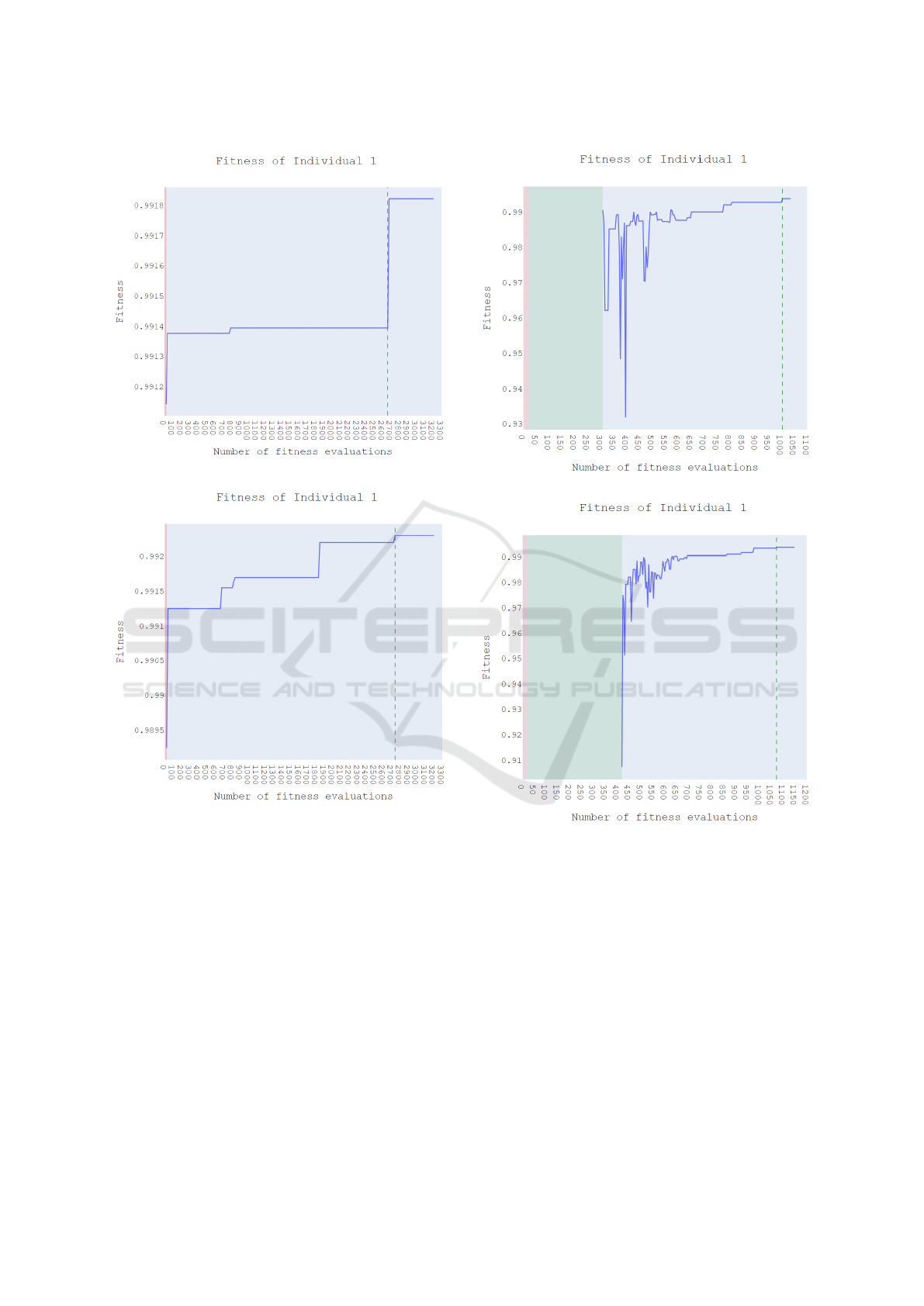
(a) Fitness of Individual 1 from Population 1.

(b) Fitness of Individual 1 from Population 2.

Figure 5: The above ﬁgures indicate the variation of ﬁtness

over number of ﬁtness evaluations during the evolutionary

process for Populations 1 and 2. The best ﬁtness for (5a) is

obtained after 2676 evaluations and that for (5b) is obtained

after 2746 evaluations. The shaded red region represents the

number of ﬁtness evaluations during the initialization of the

population.

In addition, we have observed that including nov-

elty as an objective has the effect of reducing the vari-

ance of recognition errors by an order of magnitude

compared to the pure evolutionary approach. The

proposed method involves optimizing individual solu-

tions within a constrained local neighbourhood. Thus,

we infer from this result that the proposed method ef-

fectively obtains optimal solutions belonging to dif-

ferent regions of the solution space.

(a) Fitness of Individual 1 from Population 3.

(b) Fitness of Individual 1 from Population 4.

Figure 6: The above ﬁgures indicate the variation of ﬁtness

over the local optimization process for Populations 3 and

4. The best ﬁtness for (6a) is obtained after 1004 evalua-

tions and that for (6b) is obtained after 1072 evaluations,

during the optimization phase. The shaded red region rep-

resents the number of ﬁtness evaluations during the initial-

ization and the green region represents the number of ﬁtness

evaluations during the evolutionary process until sampling

is done.

The best recognition error obtained by our method

on the MNIST test data-set was found to be 0.48%. In

comparison to related works, this reﬂects competitive

performance. However, some peer competitors have

obtained recognition error as low as 0.32%. In order

to improve performance of the CNNs evolved using

ECTA 2021 - 13th International Conference on Evolutionary Computation Theory and Applications

132

our CGP framework, we recommend the investigation

of regularization techniques, such as dropout. Also,

the evolution of recurrent structures within the CNNs

may be explored for improved performance.

Future work may explore measures of structural

similarity which act on the DAG representation of

CGP genotype, such as Graph Edit Distance (Sanfe-

liu and Fu, 1983). In addition, the method may be ap-

plied to other CNN tasks such as image segmentation.

Lastly, an investigation of alternative SLS algorithms

may yield further improvements in terms of reduced

computational cost.

ACKNOWLEDGEMENTS

We acknowledge the support of the Natural Sci-

ences and Engineering Research Council of Canada

(NSERC).

REFERENCES

Baldominos, A., Saez, Y., and Isasi, P. (2018). Evolution-

ary convolutional neural networks: An application to

handwriting recognition. Neurocomputing, 283:38–

52.

Caruana, R., Lawrence, S., and Giles, L. (2000). Overﬁt-

ting in neural nets: Backpropagation, conjugate gra-

dient, and early stopping. NIPS’00, page 381–387,

Cambridge, MA, USA. MIT Press.

Chollet, F. et al. (2015). Keras. https://keras.io.

Cover, T. and Hart, P. (1967). Nearest neighbor pattern clas-

siﬁcation. IEEE Transactions on Information Theory,

13(1):21–27.

Deb, K., Pratap, A., Agarwal, S., and Meyarivan, T. (2002).

A fast and elitist multiobjective genetic algorithm:

Nsga-ii. IEEE Transactions on Evolutionary Compu-

tation, 6(2):182–197.

D’Souza, R., Sekaran, C., and Kandasamy, A. (2010). Im-

proved nsga-ii based on a novel ranking scheme. Jour-

nal of Computing, 2.

Fernandes Junior, F. E. and Yen, G. G. (2019). Particle

swarm optimization of deep neural networks architec-

tures for image classiﬁcation. Swarm and Evolution-

ary Computation, 49:62–74.

Kingma, D. P. and Ba, J. (2017). Adam: A method for

stochastic optimization.

Kirkpatrick, S., Gelatt, C. D., and Vecchi, M. P. (1983).

Optimization by simulated annealing. Science,

220(4598):671–680.

Lecun, Y., Bottou, L., Bengio, Y., and Haffner, P. (1998).

Gradient-based learning applied to document recogni-

tion. Proceedings of the IEEE, 86(11):2278–2324.

LeCun, Y. and Cortes, C. (2010). MNIST handwritten digit

database.

Lehman, J. and Stanley, K. O. (2011). Novelty search and

the problem with objectives. In Riolo, R., Vladislavl-

eva, E., and Moore, J. H., editors, Genetic Program-

ming Theory and Practice IX, pages 37–56. Springer

New York, New York, NY.

McGhie, A., Xue, B., and Zhang, M. (2020). Gpcnn:

evolving convolutional neural networks using genetic

programming. In 2020 IEEE Symposium Series on

Computational Intelligence (SSCI), pages 2684–2691,

Canberra, ACT, Australia. IEEE.

Miller, B. and Goldberg, D. (1995). Genetic algorithms,

tournament selection, and the effects of noise. Com-

plex Syst., 9.

Miller, J. F. and Thomson, P. (2000). Cartesian genetic pro-

gramming.

Sanfeliu, A. and Fu, K.-S. (1983). A distance measure be-

tween attributed relational graphs for pattern recogni-

tion. IEEE Transactions on Systems, Man, and Cyber-

netics, SMC-13(3):353–362.

Srivastava, N., Hinton, G., Krizhevsky, A., Sutskever, I.,

and Salakhutdinov, R. (2014). Dropout: a simple way

to prevent neural networks from overﬁtting. The jour-

nal of machine learning research, 15(1):1929–1958.

Stanley, K. O., D’Ambrosio, D. B., and Gauci, J. (2009). A

Hypercube-Based Encoding for Evolving Large-Scale

Neural Networks. Artiﬁcial Life, 15(2):185–212.

Stanley, K. O. and Miikkulainen, R. (2002). Evolving Neu-

ral Networks through Augmenting Topologies. Evo-

lutionary Computation, 10(2):99–127.

Suganuma, M., Shirakawa, S., and Nagao, T. (2017). A

genetic programming approach to designing convolu-

tional neural network architectures. In Proceedings

of the Genetic and Evolutionary Computation Confer-

ence, pages 497–504, Berlin Germany. ACM.

Sun, Y., Xue, B., Zhang, M., Yen, G. G., and Lv, J.

(2020). Automatically designing cnn architectures

using the genetic algorithm for image classiﬁcation.

IEEE Transactions on Cybernetics, 50(9):3840–3854.

Sun, Y., Yen, G. G., and Yi, Z. (2019). Evolving unsuper-

vised deep neural networks for learning meaningful

representations. IEEE Transactions on Evolutionary

Computation, 23(1):89–103.

Verbancsics, P. and Harguess, J. (2015). Image classiﬁca-

tion using generative neuro evolution for deep learn-

ing. In 2015 IEEE Winter Conference on Applications

of Computer Vision, pages 488–493.

Wang, B., Sun, Y., Xue, B., and Zhang, M. (2018). Evolving

deep convolutional neural networks by variable-length

particle swarm optimization for image classiﬁcation.

In 2018 IEEE Congress on Evolutionary Computation

(CEC), pages 1–8.

Xie, L. and Yuille, A. (2017). Genetic cnn. In 2017 IEEE

International Conference on Computer Vision (ICCV),

pages 1388–1397, Venice. IEEE.

A Hybrid Evolutionary Algorithm, Utilizing Novelty Search and Local Optimization, Used to Design Convolutional Neural Networks for

Handwritten Digit Recognition

133