Event-based Pathology Data Prioritisation: A Study using Multi-variate

Time Series Classiﬁcation

Jing Qi

, Girvan Burnside

, Paul Charnley

and Frans Coenen

Department of Computer Science, The University of Liverpool, Liverpool L69 3BX, U.K.

Department of Biostatistics, The University of Liverpool, Liverpool L69 3BX, U.K.

Wirral University Teaching Hospital NHS Foundation Trust, Arrowe Park Hospital, Wirral CH49 5PE, U.K.

Keywords:

Data Prioritisation, Time Series Classiﬁcation, kNN, LSTM-RNN.

Abstract:

A particular challenge for any hospital is the large amount of pathology data that doctors are routinely pre-

sented with. Pathology result analysis is routine in hospital environments. Some form of machine learning

for pathology result prioritisation is therefore desirable. Patients typically have a history of pathology results,

and each pathology result may have several dimensions, hence time series analysis for prioritisation suggests

itself. However, because of the resource required, labelled prioritisation training data is typically not readily

available. Hence traditional supervised learning and/or ranking is not a realistic solution and some alternative

solution is required. The idea presented in this paper is to use the outcome event, what happened to a patient,

as a proxy for a ground truth prioritisation data set. This idea is explored using two approaches: kNN time

series classiﬁcation and Long Short-Term Memory deep learning.

1 INTRODUCTION

The challenge of prioritising pathology time series

data using the tools and techniques of machine learn-

ing is that, in most cases, we do not have sufﬁcient

amounts of training data, because of the clinical re-

source required to create such data, to support effec-

tive supervised learning. This means that some al-

ternative mechanism needs to be adopted. The fun-

damental idea presented in this paper is to use some

form of proxy for the training data set using meta-

knowledge about patients. More speciﬁcally using

meta-knowledge concerning the “ﬁnal destination” of

patients, the outcome event for each patient, and use

this to build a outcome event classiﬁcation system.

Three outcome events were considered: Emergency

Patient (EP), an In-Patient (IP) or an Out Patient (OP).

Then, given a new pathology result and the patient’s

pathology history, it would be possible to predict the

outcome event and then use this to prioritise the new

pathology result. For example if we predict the out-

come event for a patient to be EP, then the new pathol-

ogy result should be assigned high priority; however,

if we predict that the outcome event will be IP the new

pathology result should be assigned medium priority,

and otherwise low.

The hypothesis that this paper seeks to establish

is that there are patterns in patients’ historical lab

test results, which are markers as to where the pa-

tient “ended up” and which can hence be used for

prioritisation. To act as focus, the work presented is

directed at pathology lab test results related to renal

function, namely Urea and Electrolytes (U&E) tests.

This test provides an extra challenge in that it features

ﬁve components (tasks) each with an associated test

result value. In addition each task within a U&E test

has three values associated with it. Thus there are ﬁve

historical multi-variate time series per patient.

There are a number of multi-variate time series

classiﬁcation algorithms that could be adopted to clas-

sify time series. Two are considered in this paper: (i)

k Nearest Neighbour (kNN) (Xing and Bei, 2019) and

(ii) Long short-term memory (LSTM). The ﬁrst was

selected because it was the most frequency used al-

gorithm with respect to time series classiﬁcation. A

value of k = 1 was adopted, as suggested in (Bagnall

et al., 2017). Dynamic Time Warping (DTW) was

used as the similarity measure.

The remainder of the paper is organised as fol-

lows. Section 2 presents previous work relating to the

work in this paper. An overview of the U&E appli-

cation domain is then given Section 3, followed by a

formalism in Section 4. The two proposed approaches

to event-based prioritisation, using kNN and LSTM,

are presented in Section 5. The evaluation of the pro-

posed approaches is then presented in Section 6. Fi-

nally, in Section 7, some conclusions and directions

for future work are considered.

Qi, J., Burnside, G., Charnley, P. and Coenen, F.

Event-based Pathology Data Prioritisation: A Study using Multi-variate Time Series Classiﬁcation.

DOI: 10.5220/0010643900003064

In Proceedings of the 13th International Joint Conference on Knowledge Discovery, Knowledge Engineering and Knowledge Management (IC3K 2021) - Volume 1: KDIR, pages 121-128

ISBN: 978-989-758-533-3; ISSN: 2184-3228

121

2 PREVIOUS WORK

The prioritisation mechanism proposed in this paper

is founded on time series classiﬁcation. Many time

series classiﬁcation approaches have been proposed.

One of the most popular, and that used with respect to

the work presented in this paper, is k Nearest Neigh-

bour (kNN) classiﬁcation. The fundamental idea of

kNN classiﬁcation is to compare a previously unseen

time series, which we wish to label, with a “bank”

of time series whose labels are known, identify the k

most similar and use the labels from the k most simi-

lar to label the previously unseen time series. Usually

k = 1 is adopted because it avoids the need for any

conﬂict resolution.

Time series classiﬁcation using kNN entails two

challenges: (i) the data format for the input time se-

ries, and (ii) the nature of the similarity (distance)

measure to be used to establish similarity (Wang et al.,

2013). There are two popular time series formats:

(i) instance-based and (ii) feature-based. Using the

instance-based format the original time series format

is maintained. Using the feature-based representation,

properties of the time series are used (Wang et al.,

2008). For the work presented in this paper the in-

stance based format was used. There are a number of

similarity measure options including Euclidean, Man-

hattan and Minkowski distance measurement, but Dy-

namic Time Warping (DTW) is considered to be the

most effective with respect to the instance-based for-

mat, and offers the additional advantage that the time

series considered do not have to be of the same length

(Wang et al., 2013). For the work presented in this

paper DTW was adopted.

The recent success of deep learning offers a more

substantive way of processing time series than in the

case of traditional models. Among many deep learn-

ing techniques, Recurrent Neural Networks(RNNs)

are considered as an effective way of classifying time

series, because they allow for the processing of vari-

able length inputs and outputs by maintaining state

information across time steps. There are many ex-

amples in the literature where RNNs have been used

with respect to time series classiﬁcation; see for ex-

ample (Choi et al., 2016; Esteban et al., 2015). Long

Short-Term Memory (LSTM) networks are a popular

form of RNNs. The advantage of RNNs in general,

and LSTMs in particular, is that they have shown to

be more accurate, with respect to time series classi-

ﬁcation, then kNN. However, kNN does not require

signiﬁcant training or large amounts of training data

as in the case of RNNs (LSTMs). There are many

variations of LSTMs (Greff et al., 2016). In this pa-

per, the standard “vanilla” LSTM setup was used.

3 APPLICATION DOMAIN

The work presented in this paper is focused on the

Urea and Electrolytes (U&E) test; a commonly used

test to detect abnormalities of blood chemistry, pri-

marily kidney (renal) function and dehydration. A

U&E test is usually performed to conﬁrm normal kid-

ney function or to exclude a serious imbalance of

biochemical salts in the bloodstream. The U&E test

data considered in this paper comprised, for each test,

measurement of levels of: (i) Sodium (So), (ii) Potas-

sium (Po), (iii) Urea (Ur), (vi) Creatinine (Cr), and

(v) Bicarbonate (Bi). The measurement of each is re-

ferred to as a “task”, thus we have ﬁve tasks per test.

In other words each U&E test results in ﬁve pathology

values. It is suggested that U&E pathology results can

be prioritised more precisely if the trend of the his-

torical records is taken into consideration, therefore

providing more efﬁcient treatment for patients with a

potential risk of renal function conditions. Given a

new set of pathology values for a U&E test we wish

to determine the priority to be associated with this set

of values.

4 FORMALISM

In the context of the foregoing, the assumption is that

the training data comprises a set of pathology results,

D = {P

, P

, . . . }, where the class (event) label c for

each pathology record P

∈ D is known. As the focus

of the work is U&E test data, which comprises ﬁve

tasks (components), each record P

∈ D is of the form:

= hId, Date, Gender, T

, T

, ci (1)

Where T

to T

are ﬁve multi-variate time series rep-

resenting, in sequence, pathology results for the ﬁve

tasks typically found in a U&E test: Sodium (So),

Potassium (Po), Urea (U r), Creatinine (Cr) and Bicar-

bonate (Bi); and c is the class label taken from a set of

classes C. Each time series T

has three dimensions:

(i) pathology result, (ii) normal low and (iii) normal

high. The normal low and high dimensions indicate

a “band” in which pathology results are expected to

fall. These values are less volatile than the pathology

result values themselves, but do change for each pa-

tient over time. Thus each times series T

comprises a

sequence of tuples, of the form hv, nl, nhi (pathology

result, normal low and normal high respectively).

To derive the class label for each record P

∈ D

reference was made to the outcome event(s) associ-

ated with each patient. For the evaluation presented

later in this paper, three outcome events were consid-

ered: (i) Emergency Patient (EP), an In-Patient (IP)

KDIR 2021 - 13th International Conference on Knowledge Discovery and Information Retrieval

122

or an Out Patient (OP) which were correlated with

the priority descriptors “high”, “medium” and “low”

respectively. Hence C = {high, medium, low}.

Given a new pathology result for a patient j,

comprised of ﬁve tuples, one per task, {V

n+1

, v

n+1

, v

n+1

}, these will be incorpo-

rated into the patient record P

for the patient in ques-

tion by appending each new pathology tuple to the ap-

propriate time series T

to give {V

. . .V

n+1

The patient record P

thus becomes the “query

record”, the record we wish to label.

5 MULTI-TIME SERIES

EVENT-BASED PATHOLOGY

DATA PRIORITISATION

The fundamental idea promoted in this paper is that

pathology results can be prioritised in terms of the

trend of a given patients’ pathology. In order to val-

idate this idea, two approaches were adopted, the

kNN-DTW approach and the LSTM-RNN approach.

Each is discussed in more detail below.

5.1 Event-based Data Prioritisation

using kNN

The kNN classiﬁcation model uses a parameter k, the

number of best matches we are looking for. As al-

ready noted, k = 1 was used with respect to the eval-

uation reported later in this paper because this avoids

the need for a conﬂict resolution mechanism where

k > 1. As also noted earlier, Dynamic Time Warp-

ing (DTW) was used for similarity measurement be-

cause of its ability to operates with time series of

different length (Wang et al., 2013). The disadvan-

tage of DTW is its high computational complexity,

which is O(x× y) where x and y are the lengths of the

two time series under consideration. There are many

techniques available for reducing this time complex-

ity in the context of kNN classiﬁcation. For the work

presented here “early-abandonment” (Rakthanmanon

et al., 2012) and LB-Keogh lower bounding (Vikram

et al., 2013) were used.

The traditional manner in which kNN is applied

in the context of time series analysis is to compare

a query time series with the time series in the kNN

bank. In the case of the U&E test data prioritisation

scenario considered here the process involved ﬁve

comparisons, once for each time series in the query

record P

, T

and T

. In addition,

although traditional kNN is applied to univariate time

series; in this case three-dimensional, multi-variate,

time series were used.

For each comparison ﬁve distance measures were

obtained. With respect to the proposed kNN, the ﬁve

tasks were considered independently and the ﬁnal pri-

oritisation decided using a “High priority ﬁrst and vot-

ing second” mechanism. Given the foregoing, the ap-

plication of kNN to label P

was as follows:

1. Calculate the LB-keogh overlap for the ﬁve com-

ponent time series separately and prune all records

in D where the overlap for any one time series was

greater than a threshold ε, to leave D

2. Apply DTW, with early-abandonment to each pair

, T

∈ D

i where i indicates the U&E task.

3. Assign the class label c associated with the most

similar time series T

∈ D

to the time series T

a patient record P

4. Use the “High priority ﬁrst and voting second”

mechanism to decide the ﬁnal priority level for P

The intuitions underpinning the mechanism were:

(i) if any of the ﬁve time series T

is assigned as

high prioritisation label, the ﬁnal label for a pa-

tient record P

should be high, (ii) else the ﬁnal

label is the one that receives more than half of the

votes (given a “tiebreak” the higher level of the

two labels is assigned to the patient).

The choice of value for the lower bounding thresh-

old ε was of great importance as it affected the ef-

ﬁciency and the accuracy of the similarity search.

According to (Li et al., 2017), there is a threshold

value for ε whereby the time complexity for the lower

bounding is greater than simply using DTW distance

without lower bounding. The experiments presented

in (Li et al., 2017) demonstrated that this threshold

occurred when the value for ε prunes 90% of the time

series in D. For the evaluation presented in this paper

ε = 0.159 was used because, on average, this resulted

in 10% of the time series in D being retained.

5.2 Event-based Data Prioritisation

using LSTM-RNN

The event-based data prioritisation process founded

on LSTM commenced with the training of ﬁve LSTM

models one per task: LST M

, LST M

LST M

and DLST M

. Once we have the LSTMs

they can be used.

The overall architecture comprised three “layers”:

(i) the input layer, (ii) the model layer and (iii) the de-

cision layer. In the input layer the component time

series T

, D

and D

are extracted

from the query record P

. Thus for each task we

have a multi-variate time series T

= {V

, ...,V

Event-based Pathology Data Prioritisation: A Study using Multi-variate Time Series Classiﬁcation

123

where V − J is a tuple of the form presented earlier,

and m ∈ [l

min

, l

max

]. Where necessary each time se-

ries T

is padded to the maximum length, l

max

using

the mean values for the pathology test values, normal

low and normal high values in T

. Each time series T

is then passed to the appropriate LSTM in the model

layer. Each LSTM comprised: (i) an input layer, (ii)

an LSTM layer with two layers of LSTM cells and

(iii) an output layer. The output layer included the

Logits and Softmax components.

The last layer is the architecture is the decision

layer where the ﬁnal label is derived. After obtaining

all of the ﬁve outputs and predicted labels from the

ﬁve LSTM models, a decision logic module was used

to decide the ﬁnal prioritisation level of the patient.

The Softmax function for normalising was as follows:

|C|

k=1

∀i ∈ 1...C (2)

Where: (i) |C| is the number of classes (three in this

case) and (ii) a

is the output of the LSTM layer. Fi-

nally the following “High priority ﬁrst and voting sec-

ond” rule was applied to produce the end classiﬁca-

tion: if any one of the ﬁve LSTMS produces a pre-

diction of “High” the ﬁnal prediction is “high”, oth-

erwise average the ﬁve outputs produced by Softmax

function and then choose the class with the maximum

probability.

The adopted individual LSTM architectures com-

prises 2 hidden layers and Logits plus Softmax func-

tion in the output layer, because multi-classes classi-

ﬁcation is being undertaken. For the LSTM to op-

erate ﬁve parameters needed to be tuned during the

training process. The parameters belong to two cate-

gories: (i) optimization parameters and (ii) model pa-

rameters. The optimization parameters were: Learn-

ing rate, batch size and number of epochs. The model

parameters were the number of hidden layers and the

number of hidden units. For the optimization, Adam

optimization was chosen due to its efﬁciency and the

nature of adaptive learning rate. For ﬁnding the op-

timal parameters, cross-entropy was used as the loss

function and the parameters tuned by observing the

loss and accuracy plots of the training and validation

data.

6 EVALUATION

This section presents the evaluation of the proposed

multi-time series event-based pathology data priori-

tising approach using kNN and LSTM as described

above. The metrics used were accuracy, precision and

recall. In all cases the evaluation was conducted using

a desktop machine with a 3.2 GHz Quad-Core Intel

Core i5 processor and 24 GB of RAM. For the LSTM

a GPU laptop was used ﬁtted with a NVIDA GeForce

RTX 2060 unit. Five-fold cross validation was used

through-out. For the evaluation U&E pathology data

provided by the Wirral Teaching Hospital in Mersey-

side in the UK was used. This was used to create

three data sets: (i) D

f emale

, (ii) D

male

and (iii) D

all

(where D

all

= D

f emale

∪ D

male

). An overview of the

U&E evaluation data sets is given in Sub-section 6.1.

The objectives of the evaluation were:

1. To identify the optimum parameter settings in the

context of LSTM approach.

2. To compare the operation of the kNN and LSTM

approaches in terms of effectiveness.

3. To compare the operation of the kNN and LSTM

approaches in terms of efﬁciency (runtime).

The results with respect to each of the above are dis-

cussed in sub-sections 6.2 and 6.3 respectively.

6.1 Evaluation Dataset

The Wirral Teaching Hospital U&E pathology test

data comprised four data tables. The ﬁrst three

were event data tables: (i) Emergency Patient (EP),

(ii) Inpatient(IP) and Outpatient (OP); comprised of

180,865, 226,634 and 955,318 records respectively

and corresponding to High, Medium and Low prior-

ity. The fourth was a Laboratory (Lab) data table,

comprised of 532,801 records, holding the pathology

results; this included results for patients in the event

data tables and patients that had never visited the hos-

pital, but were treated at their local surgery. The data

sets contain patient records over a two year span. The

LAB dataset was the primary dataset used for the

evaluation reported here. The event data sets were

used for generating outcome event labels (classes) for

the time series held in the LAB dataset.

Some statistics concerning the data set are given

in Table 1. From the table it can be observed that

there is a signiﬁcant imbalance between the number

of records associated with each class, this is not an

issue when using kNN with k = 1, but it is an issue

when using LSTMs, as highly imbalanced data may

pose bias towards the majority class. An oversam-

pling technique was adopted to address this issue with

respect to the RNN training.

Each record in the LAB table, R

, representing a

pathology result for a single task in a U&E test, was

of the form:

= hID, Task, Date,Value,Unit, Max, Min, Genderi

(3)

KDIR 2021 - 13th International Conference on Knowledge Discovery and Information Retrieval

124

Table 1: U&E Data set statistics.

Event (Priority) Num. Patients

Emergency Patient (High) 255

In Patient (Medium) 123

Out Patient (Low) 3,356

Total 3,734

Where: (i) ID is the unique code for the patient, (ii)

Task is the name of the task (Sodium, Potassium,

Urea, Creatinine and Bicarbonate). (iii) Date is the

date the test was conducted, (iv) Value is the pathol-

ogy value for the task, (v) Unit is the units for the

Value, and (vi) Max and Min are the bounds for the

anticipated normal range for the Value (for the patient

and task in question, not the same for all patients).

Some data cleaning was ﬁrst undertaken, removing

patients with missing or non-numeric task values and

feature scaling to beneﬁt the faster convergence of the

LSTM.

The time series data set D = {P

, P

, . . . },

where each P

patient record was of the form

hID, TestDate, Gender, T

, T

, ci (see

Section 4), required ﬁve time series equating to the

ﬁve tasks included in the U&E test data (Sodium,

Potassium, Urea, Creatinine and Bicarbonate). The

time series were constructed by processing the data

for each patient up until an outcome event. The

values, up to and including the event value, were then

used to construct the relevant time series. If a patient

appeared in more than one event data set, for example

a patient was an “out patient” and then became an “in

patient” and ﬁnally became an “emergency patient”,

then the time series prior to the“emergency event”

was used, because the pattern of the “emergency

patient” indicates the highest priority. Also there

were a small number of patients (less than 1% of

the total data set) who did not appear in any of the

event data sets, in other words the patients remained

with their general practitioners. This group of patient

records was removed from the training data. Time

series comprised of less than three time stamps

were also removed. Each P

patient record was then

labelled according to the priority indicated by the

event value time stamp.

The ﬁnal data set, D

all

, comprised 3,734 time se-

ries; 255 high priority, 123 medium priority and 3,356

low priority, covering all ﬁve tasks. Thus there were

747 records (3,734/5) in each fold of the cross valida-

tion. The records in each fold were stratiﬁed so that

there was an equal distribution of classes in each fold.

The D

f emale

data set was comprised of 1,960 time se-

ries; 136 high priority, 55 medium priority and 1,769

low priority. The D

male

, comprised of 1,774 time se-

ries; 119 high priority, 68 medium priority and 1,587

low priority. All three data sets were used for the eval-

uation. The reason for exploring the distinction be-

tween genders was because it had been suggested that

there maybe gender differences for the prioritisations

being investigated (Halbesma et al., 2008; Tomlinson

and Clase, 2019).

Table 2: LSTM Parameter Settings for the ﬁve LSTMs (one

per task).

Para.

Task

Bo Cr Po So Ur

Learning

0.01 0.01 0.01 0.01 0.01

Rate

Batch

512 128 256 512 512

Size

Epochs 1000 1000 1000 1000 1000

Hidden

2 2 2 2 2

Layer

Hidden

32 32 16 32 32

Units

6.2 Parameter Settings for LSTM

The general way for ﬁnding the best parameters for

deep neural network models is to analyse the learning

curve and accuracy plot of the training and validation

data. The most popular learning curve used for this

purpose is loss over time. Loss measures the model

error, in other words, “how bad the performance of

the model is”. Thus, the lower the loss is, the bet-

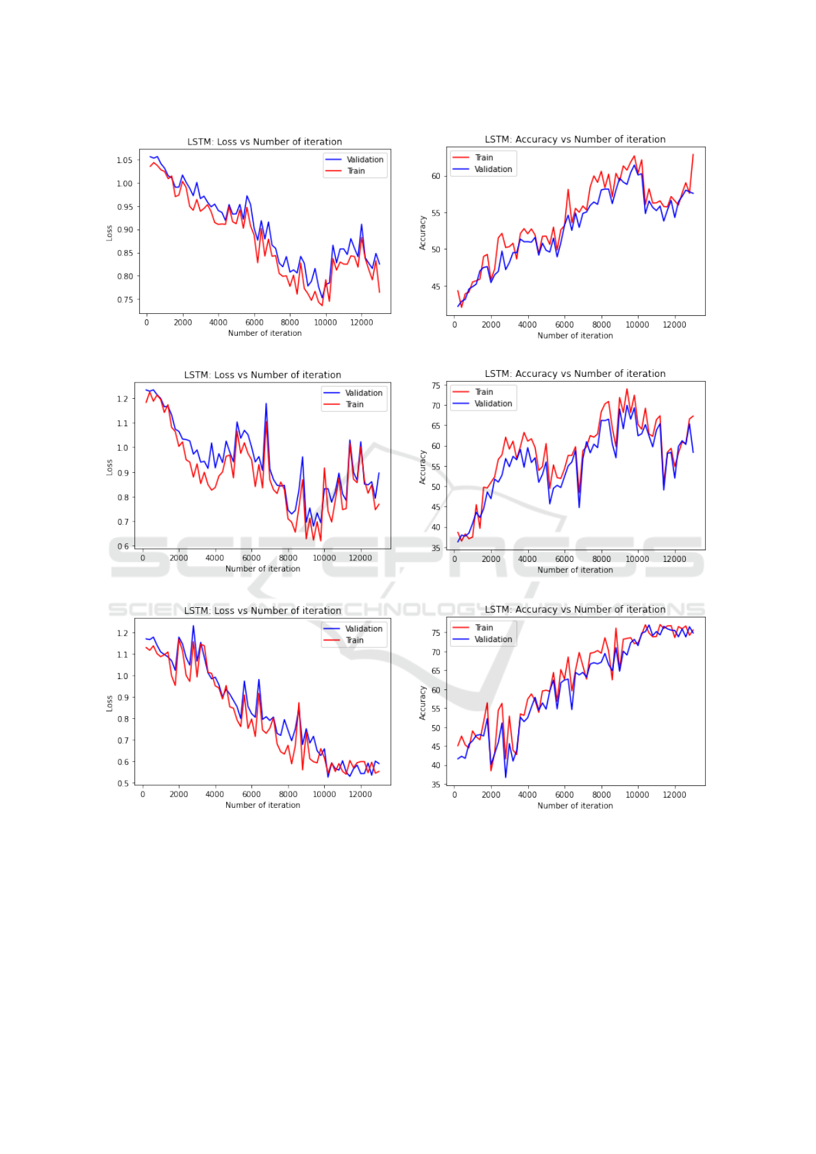
ter the model performance. Figure 1 shows the aver-

age loss and accuracy plots for each of the three data

sets considered. For each graph in Figure 1 the x-axis

gives the number of times the weights in the network

were updated, and the y-axis the loss value. From the

ﬁgures, we can observe that oscillations appear in all

of the loss and accuracy plots and that convergence is

not obvious. Possible reasons for this include: (i) the

oversampling solution for dealing with the class im-

balanced problem meant that there were insufﬁcient

sequences for the LSTM to learn from; and (ii) that

the event-based mechanism used as the proxy ground

truth of the data set may not be entirely representative.

The ﬁnal best settings for the parameters are given in

Table 2.

6.3 Comparison of Approaches

The average accuracy, precision and recall results for

each fold of the ﬁve-cross validation, for the kNN and

LSTM approaches, are given in Tables 3 and 4. Note

that the results are the average results of the three

Event-based Pathology Data Prioritisation: A Study using Multi-variate Time Series Classiﬁcation

125

(a) Loss (D

all

)

(b) Accuracy (D

all

)

f emale

)

(d) Accuracy (D

f emale

)

male

)

(d) Accuracy (D

male

)

Figure 1: Loss and Accuracy curves for the LSTM generation process.

evaluation data sets. The results of the precision and

recall for the class high are highlighted. The overall

average (Ave) and standard deviation (SD) are given

in the last two rows. Note that the SD values are low,

indicating that there is little variation across the folds.

From the table it can be seen that the RNN approach

consistently outperformed the kNN approach. A gen-

eral observation is that the precision and recall values

might be argued to be on the low side, possibly in-

dicating either: (i) that the hypothesised event-based

prioritisation approach, is not as good a predictor of

priority, as anticipated, (ii) the irregular nature (dis-

tribution of time stamps) of the time series, which

was not considered, may have an adverse effect. For

the LSTM-RNN models, the way that the class im-

balanced problem was dealt with may also have ad-

KDIR 2021 - 13th International Conference on Knowledge Discovery and Information Retrieval

126

Table 3: Average Precision and Recall (Three data set) of kNN.

Fold Num. Acc. Pre. High Pre. Medium Pre. Low Rec. High Rec. Medium Rec. Low

1 0.585 0.414 0.400 0.545 0.637 0.577 0.666

2 0.632 0.534 0.688 0.578 0.678 0.467 0.714

3 0.576 0.412 0.541 0.674 0.588 0.535 0.647

4 0.523 0.598 0.541 0.634 0.712 0.4688 0.505

5 0.566 0.444 0.384 0.598 0.541 0.487 0.785

Ave 0.576 0.480 0.510 0.605 0.631 0.507 0.663

SD 0.039 0.082 0.124 0.050 0.068 0.047 0.103

Table 4: Average Precision and Recall (Three data set) of RNN.

Fold Num. Acc. Pre. High Pre. Medium Pre. Low Rec. High Rec. Medium Rec. Low

1 0.671 0.578 0.374 0.711 0.811 0.641 0.412

2 0.642 0.475 0.552 0.735 0.758 0.468 0.577

3 0.622 0.553 0.577 0.708 0.669 0.547 0.703

4 0.608 0.615 0.714 0.699 0.712 0.563 0.697

5 0.645 0.466 0.766 0.596 0.699 0.476 0.778

Ave 0.638 0.538 0.597 0.690 0.730 0.539 0.633

SD 0.024 0.065 0.120 0.054 0.056 0.071 0.143

Table 5: Average Cross-Validation Precision and Recall of All Models.

Models Acc. Pre. High Pre. Medium Pre. Low Rec. High Rec. Medium Rec. Low

LSTM-RNN-G 0.612 0.575 0.551 0.689 0.788 0.587 0.633

LSTM-RNN-F 0.645 0.541 0.415 0.711 0.678 0.615 0.612

LSTM-RNN-M 0.657 0.648 0.825 0.670 0.724 0.415 0.654

KNN-G 0.597 0.421 0.512 0.852 0.695 0.546 0.745

KNN-F 0.565 0.387 0.673 0.678 0.645 0.498 0.698

KNN-M 0.566 0.632 0.345 0.285 0.553 0.477 0.546

Ave 0.607 0.534 0.554 0.648 0.681 0.523 0.648

versely affected performance.

Table 5 gives the overall average performance re-

sults when the three data sets are considered in isola-

tion. From the table it is interesting to see that for the

gender LSTM-RNN models, the accuracy is slightly

better than the general LSTM-RNN model, whilst this

does not feature with respect to kNN models applied

to the different data sets. Thus there is still no ob-

vious evidence to demonstrate whether the prioritisa-

tion pattern from the data is related to gender, more

investigation is needed here.

Figure 2, presents the runtimes for the kNN and

LSTM models with respect different sizes of input

data from 500 to 5, 000 increasing in steps of 500

and using one fold of the ﬁve-cross validation. From

the ﬁgure it can be seen that when using kNN with

DTW is considerably less efﬁcient than when using

the LSTM model. An improvement can be made by

changing the representation approach of the time se-

ries to optimise the data structure, so as to enable a

more efﬁcient implementation of kNN and DTW. For

the training time of a single task LSTM in a single

epoch we can see from the ﬁgure that the time efﬁ-

ciency is considerably higher than in case of the kNN

model. We can also observe that the run time line is

not linear in the case of the LSTM, as the run time is

also inﬂuenced by other parameters from the hidden

layers.

7 CONCLUSION

In this paper, a mechanism for event-based pathol-

ogy data prioritisation has been proposed for multi-

variate time series pathology result data. The mo-

tivation was the large amount of pathology data re-

ceived by hospital departments which necessitates

some form of prioritisation. The challenge was that

there is no ground-truth prioritisation data available,

because of the resource required to create this. Two

approaches were explored, one using the kNN with

DTW as a distance measurement, and one using an

LSTM mechanism. The fundamental idea underpin-

ning the event-based prioritisation is to classify newly

Event-based Pathology Data Prioritisation: A Study using Multi-variate Time Series Classiﬁcation

127

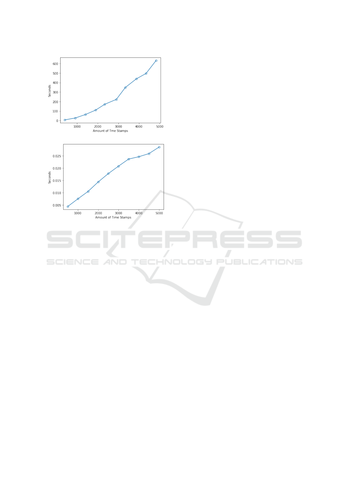
(a) Run time of kNN

(b) Run time of single task LSTM-RNN

Figure 2: Run time with different data size, (a) kNN model,

(b) LSTM-RNN model.

generated pathology data in terms of the anticipated

outcome event and then to use this outcome event

as a prioritisation marker. The proposed mechanism

was evaluated using U&E laboratory test data. The

results demonstrated that the LSTM mechanism pro-

duced the best recall and precision of 0.788 and 0.648

respectively. A criticism of the proposed RNN ap-

proach is that the process of running ﬁve LSTMs

separately is time consuming and complicated, meth-

ods using a stacked deep learning network ensemble

might be more preferable. Another criticism is that

the classiﬁcation was conducted using crisp bound-

aries which may not be the most appropriate.

REFERENCES

Bagnall, A., Lines, J., Bostrom, A., Large, J., and Keogh,

E. (2017). The great time series classiﬁcation bake

off: a review and experimental evaluation of recent

algorithmic advances. Data Mining and Knowledge

Discovery, 31(3):606–660.

Choi, E., Bahadori, M. T., Kulas, J. A., Schuetz, A., Stew-

art, W. F., and Sun, J. (2016). Retain: An interpretable

predictive model for healthcare using reverse time at-

tention mechanism. arXiv preprint arXiv:1608.05745.

Esteban, C., Schmidt, D., Krompaß, D., and Tresp, V.

(2015). Predicting sequences of clinical events by us-

ing a personalized temporal latent embedding model.

In 2015 International Conference on Healthcare In-

formatics, pages 130–139. IEEE.

Greff, K., Srivastava, R. K., Koutn

ık, J., Steunebrink, B. R.,

and Schmidhuber, J. (2016). Lstm: A search space

odyssey. IEEE transactions on neural networks and

learning systems, 28(10):2222–2232.

Halbesma, N., Brantsma, A. H., Bakker, S. J., Jansen, D. F.,

Stolk, R. P., De Zeeuw, D., De Jong, P. E., Gan-

sevoort, R. T., and for the PREVEND study group

(2008). Gender differences in predictors of the decline

of renal function in the general population. Kidney In-

ternational, 74(4):505–512.

Li, Z.-x., Wu, S.-h., Zhou, Y., and Li, C. (2017). A com-

bined ﬁltering search for dtw. In 2017 2nd Interna-

tional Conference on Image, Vision and Computing

(ICIVC), pages 884–888. IEEE.

Rakthanmanon, T., Campana, B., Mueen, A., Batista, G.,

Westover, B., Zhu, Q., Zakaria, J., and Keogh, E.

(2012). Searching and mining trillions of time se-

ries subsequences under dynamic time warping. In

Proceedings of the 18th ACM SIGKDD international

conference on Knowledge discovery and data mining,

pages 262–270.

Tomlinson, L. A. and Clase, C. M. (2019). Sex and the

incidence and prevalence of kidney disease.

Vikram, S., Li, L., and Russell, S. (2013). Handwriting and

gestures in the air, recognizing on the ﬂy. In Proceed-

ings of the CHI, volume 13, pages 1179–1184.

Wang, L., Wang, X., Leckie, C., and Ramamohanarao, K.

(2008). Characteristic-based descriptors for motion

sequence recognition. In Paciﬁc-Asia Conference on

Knowledge Discovery and Data Mining, pages 369–

380. Springer.

Wang, X., Mueen, A., Ding, H., Trajcevski, G., Scheuer-

mann, P., and Keogh, E. (2013). Experimental com-

parison of representation methods and distance mea-

sures for time series data. Data Mining and Knowl-

edge Discovery, 26(2):275–309.

Xing, W. and Bei, Y. (2019). Medical health big data clas-

siﬁcation based on knn classiﬁcation algorithm. IEEE

Access, 8:28808–28819.

KDIR 2021 - 13th International Conference on Knowledge Discovery and Information Retrieval

128