Human-error-potential Estimation based on Wearable Biometric Sensors

Hiroki Ohashi

and Hiroto Nagayoshi

Hitachi Ltd., R&D Group, Tokyo, Japan

Keywords:

Human-error Potential, Internal State, Biometric Sensing, Physiological Sensor, Wearable Sensor, Machine

Learning, Signal Processing, Activity Recognition, Shop Floor.

Abstract:

This study tackles on a new problem of estimating human-error potential on a shop ﬂoor on the basis of wear-

able sensors. Unlike existing studies that utilize biometric sensing technology to estimate people’s internal

state such as fatigue and mental stress, we attempt to estimate the human-error potential in a situation where a

target person does not stay calm, which is much more difﬁcult as sensor noise signiﬁcantly increases. We pro-

pose a novel formulation, in which the human-error-potential estimation problem is reduced to a classiﬁcation

problem, and introduce a new method that can be used for solving the classiﬁcation problem even with noisy

sensing data. The key ideas are to model the process of calculating biometric indices probabilistically so that

the prior knowledge on the biometric indices can be integrated, and to utilize the features that represent the

movement of target persons in combination with biometric features. The experimental analysis showed that

our method effectively estimates the human-error potential.

1 INTRODUCTION

Reducing human error is crucially important for al-

most all the industries to improve productivity, pre-

vent defective products, and avoid serious accidents.

The development of IoT technology has advanced

the analysis of 4M (Man, Machine, Material, and

Method) factors, but it has been especially difﬁcult to

quantitatively analyze the factor of “Man” due to its

uncertainty. The uncertainty is attributed to various

human factors including differences not only between

workers but also within workers originating from the

dynamically changing physical and mental states of

individual workers.

This study aims to develop a method to estimate

human-error potential of workers on a shop ﬂoor. The

visualization of human-error potential makes it possi-

ble to improve the working environment in various

ways such as by suggesting a short break to workers

who are found to have high error potential, by appro-

priately controlling air conditioning, and, more fun-

damentally, by reforming production lines in which

the error potential of the workers tends to be higher.

There have been relevant studies that aim to uti-

lize biometric sensing technology to estimate the in-

ternal state of humans such as fatigue (Sikander and

Anwar, 2019), mental stress (Panicker and Gayathri,

https://orcid.org/0000-0001-6970-2412

2019), drowsiness (Sahayadhas et al., 2012) (Ramzan

et al., 2019), and concentration (Uema and Inoue,

2017). The methods developed in these studies, how-

ever, cannot be trivially extended to estimate human-

error potential on shop ﬂoors for two reasons. First,

there is no formal deﬁnition of human-error potential

that can be directly used for formulating the estima-

tion problem in a computationally tractable way. Sec-

ond, the previous studies implicitly assume that target

persons are calmly seated, or at least they do not ac-

tively move, while workers usually move a lot on shop

ﬂoors, resulting in producing undesirable noise on the

measurement of the biometric sensors.

To overcome these difﬁculties, we ﬁrst propose

a novel formulation, in which the human-error-

potential estimation problem is reduced to a classi-

ﬁcation problem. We try to classify the workers’ situ-

ation into different categories including a normal sit-

uation, where human-error-potential is expected to be

low, and typical undesirable situations, where human

errors have frequently occurred according to the lit-

erature. Second, we propose a new method for esti-

mating human-error potential in a situation in which

target persons do not necessarily stay calm. The key

ideas are to model the process of calculating biomet-

ric indices probabilistically so that the prior knowl-

edge on the biometric indices can be integrated to

achieve robust estimation under noise, and to utilize

the features that represent the movement of target per-

110

Ohashi, H. and Nagayoshi, H.

Human-error-potential Estimation based on Wearable Biometric Sensors.

DOI: 10.5220/0010642400003064

In Proceedings of the 13th International Joint Conference on Knowledge Discovery, Knowledge Engineering and Knowledge Management (IC3K 2021) - Volume 1: KDIR, pages 110-120

ISBN: 978-989-758-533-3; ISSN: 2184-3228

sons in combination with biometric features. The

experimental analysis showed that our method effec-

tively estimates the human-error potential.

The contributions of this study are summarized as

follows.

1. We propose, for the ﬁrst time to the best of our

knowledge, a formulation for estimating human-

error potential on the basis of sensor data.

2. We propose a new method for estimating human-

error potential in a situation in which target per-

sons do not necessarily stay calm.

3. We experimentally veriﬁed the effectiveness of

the proposed formulation and the method for esti-

mating the human-error potential.

2 RELATED WORK

There have been intensive efforts to categorize human

errors from various aspects in order to systematically

understand them and thereby prepare effective coun-

termeasures to them. Elwyn Edward developed the

software, hardware, environment, liveware (SHELL)

model, which helps to analyze the factors that are re-

lated to human error of workers in aviation systems,

and Frank H. Hawkins later enhanced it and made it

more widely accepted (Hawkins, 1987). Swain and

Guttmann categorized the incorrect human outputs

into two major classes: omission error and commis-

sion error (Swain and Guttmann, 1983). The latter is

further divided into subcategories of selection error,

error of sequence, time error, and qualitative error.

Rasmussen presented three levels of human behavior

(skill-based, rule-based, and knowledge-based behav-

ior) to make it possible to develop separate models

for analysis (Rasmussen, 1983). Another common

method is to categorize errors into slips, lapse, and

mistakes, which represent “actions-not-as-planned”,

“failures of memory”, and “deﬁciencies or failures

in the judgemental and/or inferential processes”, re-

spectively (Reason, 1990). Although these studies

are helpful for systematically analyzing past errors or

preparing preventive measures in advance (Hale et al.,

1990)(Edmondson, 2004), they do not provide a con-

crete method for visualizing the live human-error po-

tential on a shop ﬂoor, which can dynamically change.

The relevant studies from that viewpoint are those

that have attempted to estimate people’s internal state

such as fatigue (Sikander and Anwar, 2019), mental

stress (Panicker and Gayathri, 2019), drowsiness (Sa-

hayadhas et al., 2012) (Ramzan et al., 2019), and con-

centration (Uema and Inoue, 2017). These studies

used various biometric sensing technologies together

with additional information. Wijsman et al. (Wi-

jsman et al., 2011) presented a method for detect-

ing mental stress using electrocardiogram (ECG),

respiration, skin conductance, and electromyogram

(EMG). Wang et al. (Wang et al., 2018) developed

a method for detecting a driver’s fatigue using elec-

troencephalographic (EEG) signals. Yamada and

Kobayashi (Yamada and Kobayashi, 2018) took a dif-

ferent approach for detecting fatigue on the basis of

eye-tracking data. Tsujikawa et al. (Tsujikawa et al.,

2018) and Sun et al. (Sun et al., 2018) used video

data for estimating the drowsiness. Uema and In-

oue (Uema and Inoue, 2017) developed a glasses-type

sensor for estimating the level of concentration on

the basis of electrooculography (EOG). These stud-

ies, however, cannot be trivially extended to estimate

human-error potential on shop ﬂoors mainly because

they implicitly assume that target persons are calmly

seated or at least do not actively move, whereas work-

ers usually move a lot on shop ﬂoors, resulting in

producing undesirable noise in the measurement of

the biometric sensors. Sun et al. (Sun et al., 2010)

proposed an activity-aware mental stress detection

method by using an accelerometer in combination

with ECG and galvanic skin response (GSR) sensors,

but the activities involved in their study were limited

to rather simple ones, namely, sitting, standing, and

walking.

The present study proposes a way to formulate

the human-error-potential estimation as a classiﬁca-

tion problem, standing upon the characteristics of the

human-error potential that have been revealed in the

above-mentioned works. Then we propose a new

method for estimating human-error potential in a sit-

uation in which target persons work on a pseudo in-

dustrial operation.

3 FORMULATION OF

HUMAN-ERROR-POTENTIAL

ESTIMATION

3.1 Formulation based on Major Cause

of Human Errors

As described in Hawkins’s SHELL model (Hawkins,

1987) and Swain and Guttmann’s performance shap-

ing factor (PSF) (Swain and Guttmann, 1983),

human-error is caused by various factors including

not only the worker in question, but also other work-

ers, environment, software, and hardware. Ideally, all

these factors should be sensed and taken into account

when estimating human-error potential, but this study

Human-error-potential Estimation based on Wearable Biometric Sensors

111

focuses only on the worker in question, which is nat-

urally deemed most important, as the ﬁrst step and

leaves the other factors for future works. To make the

model as general as possible without relying on a spe-

ciﬁc task’s characteristics, we focus on the possible

root cause attributed to general psychological char-

acteristics rather than focusing on the resultant cate-

gorization such as slip-lapse-mistake (Reason, 1990),

and omission-commission (Swain and Guttmann,

1983). In terms of the skill-rule-knowledge (SRK)

model by Rasmussen (Rasmussen, 1983), we focus

on the factor of “skill” since rule and knowledge are

not expected to dynamically change on shop ﬂoors

and therefore do not have to be sensed in a live

manner. Among the skill-based errors, the statistics

by Williamson et al. (Williamson et al., 1993), who

studied 2000 incident reports, showed that “inatten-

tion” and “haste” were the major contributing factors.

Inattention was found to be closely related to multi-

tasking by Ralph et al. (Ralph et al., 2014).

Standing upon these research outcomes, we at-

tempt to build a model that can detect the situations

where human-error tends to occur more frequently

according to the statistics. In this view, we can re-

duce the human-error-potential estimation problem to

a classiﬁcation problem of a worker’s situation into a

normal situation and the situation where human-error

potential is deemed higher than usual. More formally,

we formulate the problem as the classiﬁcation of three

situations: a worker is working normally, in a hurry,

and has to multi-task. We call the three conditions the

normal condition, time-pressure condition, and multi-

task condition, respectively.

3.2 Task Setting

We selected the replacement of a desktop PC’s SSD

as the experimental task because it contains basic op-

erations that are commonly done in a wide variety of

shop ﬂoors, e.g., screw tightening, wiring, and assem-

bly. The speciﬁc procedure of the task is as follows:

remove the screws of the side cover of the PC by

hand, remove the side cover, pull out the SSD mount,

unplug the cables attached to the SSD, remove the

screws using a screwdriver to detach the SSD from

the mount, replace the SSD with a new one, install

the screws to attach the new SSD to the mount using

the screwdriver, plug the cables into the SSD, place

the SSD mount back to the original position, and in-

stall the screws to attach the side cover (see Figure

1). Hereinafter, we call one series of this procedure

a “trial”. Trials lasted three minutes on average, but

they differed depending on the conditions and sub-

jects.

Figure 1: The SSD replacement task. Left: the video from

eye-tracking glasses, where the purple circle denotes the es-

timated gaze location. Right: the video from a ﬁxed camera.

In the time-pressure condition, we and asked the

subjects to ﬁnish the trial within a deﬁned time limit.

To increase the pressure, we told them the elapsed

time every 30 seconds and told them every 10 seconds

in the last 30 seconds. In the multi-task condition, we

gave them mental arithmetic problems of two digit

addition and subtraction. We read out the problems

and the subjects had to answer out loud while work-

ing on the SSD-replacement task. We did not give a

time limit for these math questions, or any penalty for

wrong answers.

3.3 Sensor Selection

We use a video camera, which does not require any

additional effort from workers for sensing. In addi-

tion, we use wearable ECG, EEG, EOG, eye-tracking

sensor, and accelerometer since they were found to

be useful for estimating internal states of humans in

the previous studies reviewed in section 2. GSR sen-

sors were also found to be useful, but we did not

use one since we found it signiﬁcantly interfered with

the task in a preliminary experiment. The sensors

used in the experiment are Logicool HD Pro Webcam

C920 (a camera for third-person-view video), SMI

Eye-Tracking Glasses (ETG) (a glasses-type cam-

era for ﬁrst-person-view video and gaze information),

TicWatch Pro (a smartwatch for acceleration data and

heart rate data), biosignalsplux (a wearable biometric

sensor for ECG and EOG data), and MindWave Mo-

bile 2 (a mobile brain-wave headset for EEG data).

Figure 2 shows these sensors.

4 ESTIMATION METHOD

4.1 Feature Extraction

This section explains the feature extraction method

for the human-error-potential estimation. First, sec-

tion 4.1.1 outlines the overall strategy for feature ex-

traction. Then, section 4.1.2 explains how to robustly

calculate important biometric indices using noisy sen-

KDIR 2021 - 13th International Conference on Knowledge Discovery and Information Retrieval

112

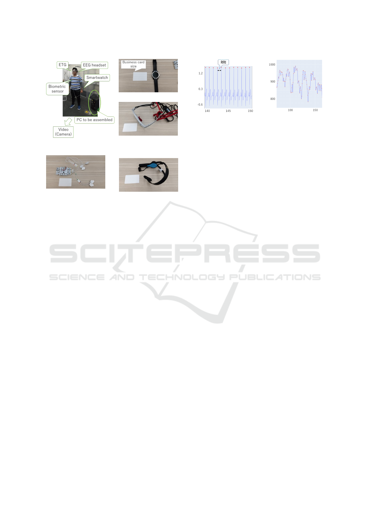
(a) Subject with all sensors.

(b) Smartwatch.

(ETG).

(d) Wearable biometric

sensor.

(e) Brain-wave headset.

Figure 2: Sensors used in experiment.

sor data. Finally, section 4.1.3 introduces the features

that represent the body movement.

4.1.1 Overall Strategy

The raw signals of ECG, EOG, and EEG data are not

usually used for the analysis. Alternatively, certain

kinds of processing such as peak detection and fre-

quency domain analysis are ﬁrst applied, and higher

level indices such as heart rate, blink frequency,

and signal intensity of a speciﬁc frequency of brain

waves are commonly used. This section outlines how

we process the data from sensors introduced in sec-

tion 3.3 to calculate such basic biometric indices. The

detailed formulation for dealing with sensor noise will

be given in section 4.1.2.

ECG data usually have periodic cycles that cor-

respond to the heart beat as shown in Figure 3(a).

We ﬁrst detect peaks, called R waves represented by

red circles in the ﬁgure, and calculate the intervals of

the R waves, which are called RR intervals, or RRI

for short (Figure 3(b)). We then extract the follow-

ing ECG-related features per trial: the mean RRI over

each trial, the strength of low frequency signals (4 Hz

≤ f < 15 Hz) of RRI wave called LF, that of high

frequency signals (15 Hz ≤ f ) called HF, and the

ratio LF/HF. HF and LF are widely used as indica-

tors of the cardiac parasympathetic nerve activity and

that of both parasympathetic and sympathetic compo-

nents, respectively.

We apply the similar feature extraction to smart-

watch data. TicWatch Pro provides heart rate data,

(a) Example of ECG data.

(b) Example of RRI.

Figure 3: Example of ECG data and its RR interval (when

a subject is staying calm). x axis: time (s), y axis: electric

potential (mV) for (a) and interval (ms) for (b).

which correspond to 60/RRI, every second. There-

fore, we calculate RRI on the basis of the heart rate

data and extract the mean RRI, LF, HF, and LF/HF in

the same way as described above.

EOG data show sharp peaks when a subject blinks.

Therefore, we ﬁrst detect these peaks and use the av-

erage frequency of blinks (times/minute) over each

trial as a feature. The details of the peak detection

method will be given in section 4.1.2.

The SMI ETG provides various eye-activity in-

formation including the gaze location in each video

frame, and the eye-event information such as visual

intake, saccade, and blink. We extract the following

features: the standard deviation of the gaze location

in horizontal and vertical directions, the mean and the

standard deviation of the distances of gaze location

between the two consecutive frames, the frequency of

the distance being larger than a threshold, the ratio of

visual-intake event, and the ratio of saccade event. We

do not use the blink event information as we found in

a preliminary experiment that it was not accurate.

The API of Mindwave Mobile 2 provides the sig-

nal strength of δ wave (1-3 Hz), θ wave (4-7 Hz),

low-α wave (8-9 Hz), high-α wave (10-12 Hz), low-

β wave (13-17 Hz), high-β wave (18-30 Hz), low-γ

wave (31-40Hz), mid-γ wave (41-50 Hz), the score

of concentration, and the score of meditation. These

measurements are provided every second. We use the

mean and standard deviation over each trial as the fea-

tures of EEG data.

The acceleration data obtained by the smartwatch

are ﬁrst converted into a movement feature using the

method described in section 4.1.3. Then we calculate

its mean over each trial. Additionally, we subtract the

mean norm of the acceleration data from the raw ac-

celeration data and then convert the result and calcu-

late the mean in the same way as above. This is for

getting rid of the factor of gravity acceleration.

The video data of a ﬁxed camera are ﬁrst con-

verted into movement features in a way that is de-

scribed in section 4.1.3 and the mean over each trial

is used as video features.

Human-error-potential Estimation based on Wearable Biometric Sensors

113

Figure 4: Example of ECG data in SSD-replacement task.

Finally, we convert all the features described

above into the deviation from the values in the calm

state by subtracting the mean values of each feature

in the calm state. This is for reducing the between-

subject bias. The effect of this pre-processing will be

discussed in section 5.4.

4.1.2 Calculation of Basic Biometric Indices

under Noise

Wearable biometric data such as ECG and EOG data

easily suffer from noise caused by body movement.

For example, ECG data show clear peaks (R wave)

when a subject stays calm (Figure 3(a)), but it be-

comes difﬁcult to accurately detect an R wave when

a subject moves as shown in Figure 4. We propose

a method for robustly calculating biometric indices

such as RRI by formulating the calculation process

using a probabilistic model, which can take the prior

knowledge about each biometric index into account.

We explain the method by using calculation of RRI

based on ECG data as an example.

Let x

denote the ECG measurement at time t and

deﬁne a set of the measurement as X

≡ {x

}

t=t

Let t

(n)

denote the timestamp of observing the n-th

R wave, and let y

(n)

denote the n-th RRI value. Note

that y

(n)

= t

(n+1)

−t

(n)

holds by the deﬁnition of RRI.

Let T be the length of ECG measurement sequence,

then the (n+1)-th RRI given a sequence of ECG mea-

surement X

and RRIs up to the n-th is modeled as

follows.

p(y

(n+1)

(n)

,...,y

(1)

)

= p(y

(n+1)

(n)

,...,y

(1)

) (1)

p(X

(n+1)

(n)

,...,y

(1)

) (2)

p(y

(n+1)

(n)

,...,y

(1)

)

(3)

p(X

(n+1)

(n)

,...,y

(1)

) (4)

p(y

(n+1)

(n)

,...,y

(1)

In equation (1), we used the assumption that the

RRIs up to the (n − 1)-th do not matter if the n-th

R wave is given. Z and Z

in equations (2) and (4),

respectively, are constant values for normalization.

p(X

(n+1)

(n)

,...,y

(1)

) in equation (4) de-

notes the probability of observing a sequence of

ECG measurement X

(n+1)

when an R wave, or peaks

of ECG data, are observed at time

(n+1)

= t

(1)

∑

n+1

i=1

(i)

. This probability is expected to be higher if

the ECG measurement at time

(n+1)

is high. There-

fore, we model it as follows.

p(X

(n+1)

(n)

,...,y

(1)

) =

(n+1)

)

, (5)

where C

is a normalization constant, and α is a hy-

perparameter. p(y

(n+1)

(n)

,...,y

(1)

) in equation (4)

represents the probability of the (n + 1)-th RRI value

being y

(n+1)

given RRIs up to the n-th, and we model

it as follows.

p(y

(n+1)

(n)

,...,y

(1)

)



N (y

(n)

,σ

) + βN (µ

(n)

,σ

) + γg(y

(n+1)

)



(6)

where N (y

(n)

,σ

) and N (µ

(n)

,σ

) denote a normal

distribution with mean y

(n)

and variance σ

, and that

of mean µ

(n)

∑

i=1

and variance σ

, respectively.

They model the prior knowledge that RRIs usually

do not drastically change compared with the previous

observation, and the mean value of the past observa-

tions. C

is a normalization constant, and β and γ are

hyperparameters. We deﬁne g(y

(n+1)

) as follows.

g(y

(n+1)

) =

∑

(n)

( f )

(n)



(n+1)



, (7)

where h

( f ) represents the signal strength of fre-

quency f in sequential data X

, which we model by

fast Fourier transform (FFT) applied to X

Finally, the (n + 1)-th RRI y

(n+1)

is estimated as

follows.

(n+1)

= argmax

ˆy

(n+1)

∈Y

(n+1)

p( ˆy

(n+1)

(n)

,...,y

(1)

), (8)

where Y

(n+1)

= {y

(n+1)

min

< y

(n+1)

< y

max

∩ x

(n)

(n+1)

∈ M}. Here y

min

max

are the minimum and

maximum possible RRI values that we preliminarily

deﬁne, and M is a set of local maxima of ECG values.

We use the same formulation for blink detection

with EOG data except that we introduce a uniform

distribution for equation (6) since it is not reasonable

to assume strong periodicity in blink detection.

KDIR 2021 - 13th International Conference on Knowledge Discovery and Information Retrieval

114

4.1.3 Extraction of Movement Feature

We extract features related to subjects’ body move-

ment using acceleration data of smartwatch and video

data of a ﬁxed camera, and use them in the human-

error-potential estimation method so that the method

can take the body movement into account.

Let (a

x,t

y,t

z,t

) denote the readings of a three-

axis accelerometer of a smartwatch at time t. We de-

ﬁne the movement features calculated on the basis of

acceleration data as follows.

(acc)

x,t

+ a

y,t

+ a

z,t

(9)

To extract video-based movement features, we

ﬁrst use a method proposed by Pavllo et al. (Pavllo

et al., 2019) to acquire a set of 3D locations of each

body joint {(l

(1)

,...,l

(J)

)}

t=1

, where l

(i)

represents

the i-th body joint’s 3D coordinate (l

( j)

x,t

( j)

y,t

( j)

z,t

) at

time t. The 3D coordinates are relative to the root

joint. We set J to be 17, which is a default value in the

previous work. We deﬁne the movement features cal-

culated on the basis of video data from a ﬁxed camera

as follows.

(video, j)



( j)

x,t

− l

( j)

x,t−1





( j)

y,t

− l

( j)

y,t−1





( j)

z,t

− l

( j)

z,t−1



(10)

Note that these features are calculated joint-wise,

which results in J features being acquired.

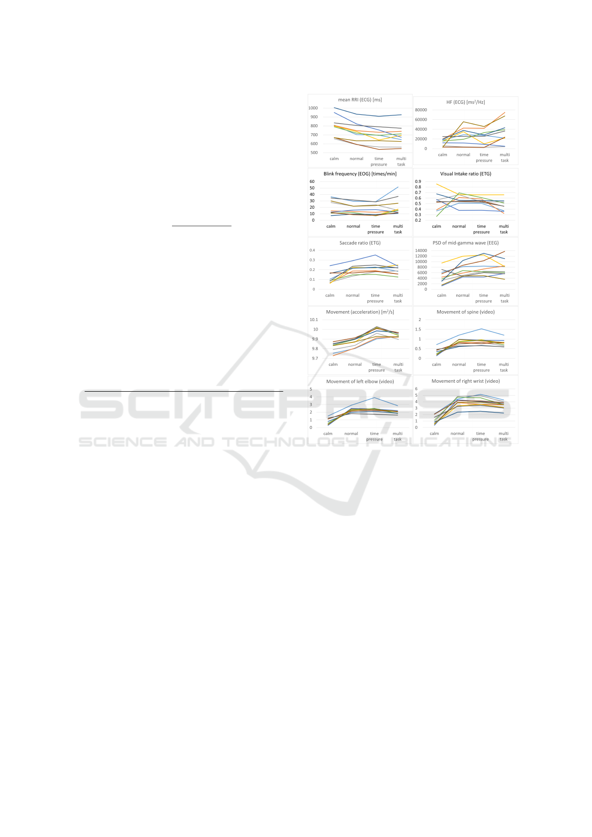
4.2 Feature Selection

We can obtain 55 different features in total by the fea-

ture extraction method described in section 4.1. Al-

though it may be possible to make the model learn

sufﬁciently well using all the 55 features if there

are enough training data, the model may suffer from

over-ﬁtting if the available training data are limited.

Therefore, we analyzed each feature in detail and

selected a set of features that showed a noticeable

tendency depending on the task conditions (normal,

time-pressure, and multi-task). As a consequence of

the analysis, we ended up selecting the 10 features

shown in Figure 5.

4.3 Classiﬁcation Model

We use neural network for the classiﬁcation model

unless otherwise stated. We use a simple fully con-

nected network rather than convolutional neural net-

works (CNN) and recurrent neural networks (RNN)

since it is not reasonable to assume locality and other

Figure 5: Ten selected features.The different colors corre-

spond to different subjects. Note that visual intake ratio and

saccade ratio have only nine subjects’ data because a subject

could not wear ETG due to an eyesight problem.

speciﬁc dependencies among the features described

in section 4.2. We will discuss the models other than

neural networks in section 5.4.

5 EVALUATION

5.1 Experimental Settings

We conducted an experiment to verify the effective-

ness of the proposed method with 10 subjects. The

experiment was conducted in a lab environment with

lab members. The experiment on a real shop ﬂoor

with real workers is one of our future works.

The overall experimental procedure is shown in

Figure 6. First, we explained the experiment to the

subjects. Then to eliminate the learning effect, they

practiced the SSD-replacement task without attach-

Human-error-potential Estimation based on Wearable Biometric Sensors

115

ing any sensors until they were sufﬁciently familiar

with the task. After they become conﬁdent doing the

task, we attached the wearable sensors and synchro-

nized all the sensors, calibrated the sensors if nec-

essary, and tested the connection. Then we let the

subjects be seated on chairs and asked them to stay

calm. We collected sensor data during this calm state.

Then the subjects practiced the task again with sen-

sors attached and conﬁrmed that the sensors did not

disturb them in the task. We collected three trials

per condition (normal, time-pressure, multi-task), re-

sulting in nine trials per subject in total. We let the

subjects take a short break after every trial. We col-

lected sensor data in this break time as well for us-

ing them as measurement in the calm state. After ﬁn-

ishing the ﬁrst trial (e.g., normal condition) and the

subsequent short break, subjects worked on another

condition (e.g., time-pressure) and took a short break

again. Then they worked on the remaining condition

(e.g., multi-task) and took a short break. Hereinafter,

we call this set of three sequential trials a “cycle”.

They repeated this cycle three times. We let a one-

third of the subjects start with the normal condition,

another third start with the time-pressure condition,

and the rest start with the multi-task condition for the

counterbalance. One trial usually took from two to

four minutes, and the whole experiment including the

preparation took approximately two hours per subject.

5.2 Evaluation Protocol

We evaluated the performance by three-fold cross val-

idation, in which we split the data by aforementioned

cycles, unless otherwise stated. More speciﬁcally, we

used the data from two cycles for training and used

the data from the other cycle for test, and repeated

this three times with different combinations of train-

ing and test data. This resulted in 6 trials from each

subject for training data and the remaining 3 trials

from each subject for test data, ending up with 60 tri-

als in total for training data and 30 trials in total for

test data. We used the mean accuracy of this three-

fold cross validation for the basic evaluation metric.

5.3 Implementation Details

We optimized the hyperparameters including learning

rate, learning schedule, number of layers, and num-

ber of nodes using the TPE algorithm (Bergstra et al.,

2011) with Optuna (Akiba et al., 2019). As a result,

we set the number of hidden layers to 3 and the num-

ber of nodes in each layer to 200, 50, and 50. The

initial learning rate was 0.03, and it was decayed by

multiplying 1/t

0.5

at the t-th epoch. The hyperparam-

Table 1: Evaluation result. Time: time-pressure condition,

Multi: multi-task condition, GT: ground truth.

Estimated

Normal Time Multi Total

Normal 7.3 2.3 0.3 10

Time 2.3 6.7 1.0 10

Multi 0.3 1.3 8.3 10

Total 10.0 10.3 9.7 30

Table 2: Comparison of feature pre-processing methods.

Pre-processing 3 classes 2 classes

Absolute 73.3 81.1

Relative 74.4 82.2

eters of models other than neural networks compared

in Table 5 were also optimized in the same way. If

a feature value was missing, we interpolated it with

the median value of the feature value over training

data. All the features were normalized by subtracting

means of each feature in the training data and dividing

them by standard deviations.

5.4 Results and Discussion

Main Result. Table 1 shows the main evaluation re-

sults. The overall accuracy was 74.4% (=67/90), and

the accuracy of binary classiﬁcation between normal

condition and abnormal conditions, where human-

error tends to occur more frequently was 82.2%

(=74/90). The table shows that the multi-task con-

dition was more clearly distinguishable from the nor-

mal condition than the time-pressure condition was.

This observation agrees with the fact that all the sub-

jects said that they felt the multi-task condition was

the most difﬁcult and the normal condition was the

easiest.

Analysis on Feature Pre-processing. Table 2

shows the effect of feature pre-processing described at

the end of section 4.1.1. “Absolute” denotes the result

obtained by using all the features directly, whereas

“Relative” denotes the result obtained by converting

features into the deviation from the values in the calm

state by subtracting the mean values of each feature in

the calm state. As the table indicates, “Relative” gave

slightly better performance than “Absolute”. We think

this is because different subjects have different base

values for biometric indices, and using values relative

to the calm states reduces this between-subject bias,

ending up in enabling us to focus more on the differ-

ence in the conditions.

KDIR 2021 - 13th International Conference on Knowledge Discovery and Information Retrieval

116

Figure 6: Experimental procedure.

Table 3: Ablation for the feature selection and the move-

ment feature. FS: the feature selection method described

in section 4.2. If this is unchecked, results are based on all

the available features without applying the feature selection.

MF: the movement features described in section 4.1.3. If

this is unchecked, results are only based on the biometric-

sensor data without using the movement features. #F: the

number of used features. 3 classes: normal, time-pressure,

and multi-task condition, 2 classes: normal condition and

abnormal condition where human-error tends to occur more

frequently.

# FS MF #F 3 classes 2 classes

1 36 56.5 71.1

2 X 6 70.0 78.9

3 X 55 61.1 65.6

4 X X 10 74.4 82.2

Ablation Study for the Feature Selection and the

Movement Feature. Table 3 shows the ablation

study for the feature selection method described in

section 4.2 and the movement features described in

section 4.1.3. The effectiveness of the feature selec-

tion is demonstrated by comparing #1 with #2, and #3

with #4. This suggests the importance of excluding

unnecessary features probably because the available

training data were small. Similarly, the effectiveness

of the movement feature is demonstrated by compar-

ing #1 with #3, and #2 with #4. This suggests the

importance of taking into account the information of

body movement when attempting to estimate human-

error potential, and possibly other psychophysiologi-

cal indices as well, in a situation where target subjects

do not stay calm.

Analysis on Feature-selection Methods. Table 4

compares different feature selection methods. #1 de-

Table 4: Comparison of different feature-selection methods.

# Feature selection #F 3 classes 2 classes

1 All features 55 61.1 65.6

2 PCA 10 61.1 65.6

3 Greedy 7 65.6 68.9

4 Analysis-based 10 74.4 82.2

notes the result obtained by using all the features

without applying any feature selection method. Note

that the movement features are also included. #2 de-

notes the result obtained by reducing the number of

dimensions to 10 with principal component analysis

(PCA). Interestingly, #2 did not result in better accu-

racy than #1. This may be because the neural network

could learn the (linear) transform that was equivalent

to PCA in the ﬁrst layer. #3 is the result obtained by

selecting features greedily (see Algorithm 1 for de-

tails). #4 is the result obtained by using the manual

feature selection described in section 4.2. Although

the greedy feature selection gave slightly better results

than #1 and #2, the analysis-based selection resulted

in much better accuracy. The result suggests the effec-

tiveness of traditional feature engineering in this ﬁeld

especially when the number of candidate features is

relatively low.

Analysis on Classiﬁcation Models. Table 5 com-

pares different classiﬁcation models. We found the

neural network worked the best. Note that the 10

manually selected features are used for all the mod-

els.

Analysis on Sensors. Table 6 shows the perfor-

mance depending on the available sensors. For the de-

ployment on shop ﬂoors, subjects, or workers, should

Human-error-potential Estimation based on Wearable Biometric Sensors

117

Algorithm 1: Greedy feature selection.

Input : F – a set of features

m– a classiﬁcation model

N – the maximum number of

features to be selected

Output: BF – best features

1 SF ← {}// a set of selected features

2 n ← 1

3 a

best

← −1

4 for n ≤ N do

5 a

(n)

best

← −1

6 for f in F do

7 a ← m (SF ∪ { f })

8 if a > a

(n)

best

then

9 a

(n)

best

← a

10 f

selected

← f

11 end

12 end

13 SF ← SF ∪ { f

selected

}

14 F ← F \ { f

selected

}

15 if a

(n)

best

> a

best

then

16 BF ← SF

17 a

best

← a

(n)

best

18 end

19 end

Table 5: Comparison of different classiﬁcation methods.

Classiﬁcation method 3 classes 2 classes

Gaussian Na

ıve Bayes 55.6 67.8

Decision Tree 65.6 72.2

k nearest neighbor 66.7 74.5

Random Forest 68.9 75.6

Support Vector Machine 72.2 81.1

Neural network 74.4 82.2

attach as few sensors as possible so that the sensors

do not disturb their work. The ideal scenario is to use

only a ﬁxed camera, which does not disturb workers at

all, but this was found to be unrealistic from the view-

point of accuracy (#1). The next reasonable scenario

is to use a smartwatch alone (#2) or in combination

with a ﬁxed camera (#3). However, the accuracies in

these conditions were still not satisfactory. Adding

EOG (#4), EEG (#5), and ETG (#6) one by one did

not improve the performance compared with using

only a ﬁxed camera and a smartwatch. In contrast, us-

ing an ECG sensor in combination with a ﬁxed cam-

era and a smartwatch achieved signiﬁcantly better re-

sults. This result suggests that it is very important to

include features calculated on the basis of ECG sig-

nals such as mean RRI and HF and indirectly implies

that the proposed method for calculating biometric in-

dices under movement noise worked well.

Analysis on the Generalization to a New Worker.

To verify the generalizability of the proposed model

to new workers, we evaluated the performance in

leave-one-subject-out cross validation. The model

was trained with nine subjects’ data and tested with

the remaining subject’s data. We repeated this evalu-

ation nine times by changing the subject whose data

were used for the test. Note that we excluded one sub-

ject’s data from testing since the ETG data of the sub-

ject were completely missing. This was because the

subject could not wear the ETG due to an eye sight

problem.

We report the averaged results of all the nine valid

subjects in Table 7. Note that the total number of tri-

als does not add up to nine because we excluded some

trials due to invalid data that could not be interpolated.

The overall accuracy decreased to 58.6%. This means

that the features used in this study have certain de-

pendencies on individual subjects, and it is difﬁcult

to use a model trained with one subject’s data to es-

timate the human-error potential of another subject.

Finding more subject-independent features is one of

our future works. If this result is seen from the other

side, however, it means that we may be able to achieve

even better performance than the results in Table 1 if

we can collect sufﬁcient training data from a worker

and build a customized model for that worker.

The accuracy of the binary classiﬁcation also de-

creased, but it stayed relatively high, which was

71.4%, suggesting the model is somewhat effective

at least for the binary classiﬁcation to some extent.

6 CONCLUSIONS

This study tackled on a new problem of estimating

human-error potential on the basis of wearable sen-

sors, aiming at reducing the human errors on a shop

ﬂoor. Unlike existing studies, we have attempted

to estimate the human-error potential in a situation

where a target person does not stay calm, which is

much more difﬁcult as sensor noise signiﬁcantly in-

creases. We proposed a novel formulation, in which

the human-error-potential estimation problem is re-

duced to a classiﬁcation problem, and introduced a

new method that can be used for solving the classiﬁ-

cation problem even with noisy sensing data. The ex-

perimental analysis demonstrated the effectiveness of

our method for estimating the human-error potential.

In addition, we found that ECG data played an im-

KDIR 2021 - 13th International Conference on Knowledge Discovery and Information Retrieval

118

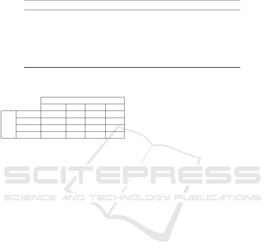
Table 6: Comparison of performances by different combinations of sensors.

# Fixed camera Smart watch EOG EEG ETG ECG 3 classes 2 classes

1 X 51.1 66.7

2 X 53.3 67.8

3 X X 56.7 66.7

4 X X X 52.2 67.8

5 X X X 53.3 70.0

6 X X X 53.3 72.2

7 X X X 68.5 75.8

8 X X X X X X 74.4 82.2

Table 7: Evaluation result of leave-one-subject-out cross

validation. Time: time-pressure condition, Multi: multi-

task condition, GT: ground truth.

Estimated

Normal Time Multi Total

Normal 1.67 0.44 0.56 2.67

Time 0.67 1.22 0.44 2.33

Multi 0.56 0.56 1.67 2.78

Total 2.89 2.22 2.67 7.78

portant role in estimating human-error potential. Our

future work includes generalizing out method to new

workers by ﬁnding out subject-independent features.

REFERENCES

Akiba, T., Sano, S., Yanase, T., Ohta, T., and Koyama, M.

(2019). Optuna: A next-generation hyperparameter

optimization framework. In International conference

on knowledge discovery & data mining.

Bergstra, J., Bardenet, R., Bengio, Y., and K

egl, B. (2011).

Algorithms for hyper-parameter optimization. In 25th

annual conference on neural information processing

systems (NIPS).

Edmondson, A. C. (2004). Learning from mistakes is easier

said than done: Group and organizational inﬂuences

on the detection and correction of human error. The

Journal of Applied Behavioral Science, 40(1):66–90.

Hale, A., Stoop, J., and Hommels, J. (1990). Human er-

ror models as predictors of accident scenarios for de-

signers in road transport systems. Ergonomics, 33(10-

11):1377–1387.

Hawkins, F. H. (1987). Human Factors in Flight. Ashgate

Publishing.

Panicker, S. S. and Gayathri, P. (2019). A survey of ma-

chine learning techniques in physiology based mental

stress detection systems. Biocybernetics and Biomed-

ical Engineering, 39(2):444–469.

Pavllo, D., Feichtenhofer, C., Grangier, D., and Auli, M.

(2019). 3D human pose estimation in video with tem-

poral convolutions and semi-supervised training. In

Conference on Computer Vision and Pattern Recogni-

tion (CVPR).

Ralph, B. C., Thomson, D. R., Cheyne, J. A., and Smilek,

D. (2014). Media multitasking and failures of at-

tention in everyday life. Psychological research,

78(5):661–669.

Ramzan, M., Khan, H. U., Awan, S. M., Ismail, A., Ilyas,

M., and Mahmood, A. (2019). A survey on state-of-

the-art drowsiness detection techniques. IEEE Access,

7:61904–61919.

Rasmussen, J. (1983). Skills, rules, and knowledge; signals,

signs, and symbols, and other distinctions in human

performance models. IEEE transactions on systems,

man, and cybernetics, SMC-13(3):257–266.

Reason, J. (1990). Human Error. Cambridge University

Press.

Sahayadhas, A., Sundaraj, K., and Murugappan, M. (2012).

Detecting Driver Drowsiness Based on Sensors: A

Review. Sensors, 12(12):16937–16953.

Sikander, G. and Anwar, S. (2019). Driver Fatigue Detec-

tion Systems: A Review. IEEE Transactions on Intel-

ligent Transportation Systems, 20(6):2339–2352.

Sun, F.-T., Kuo, C., Cheng, H.-T., Buthpitiya, S., Collins, P.,

and Griss, M. (2010). Activity-aware Mental Stress

Detection Using Physiological Sensors. In Interna-

tional conference on Mobile computing, applications,

and services, pages 282–301. Springer.

Sun, M., Tsujikawa, M., Onishi, Y., Ma, X., Nishino, A.,

and Hashimoto, S. (2018). A neural-network-based

investigation of eye-related movements for accurate

drowsiness estimation. In International Conference

of the IEEE Engineering in Medicine and Biology So-

ciety (EMBC), pages 5207–5210.

Swain, A. D. and Guttmann, H. E. (1983). Handbook of

human reliability analysis with emphasis on nuclear

power plant applications. NUREG/CR-1278, SAND

80-0200.

Tsujikawa, M., Onishi, Y., Kiuchi, Y., Ogatsu, T., Nishino,

A., and Hashimoto, S. (2018). Drowsiness estimation

from low-frame-rate facial videos using eyelid vari-

ability features. In International Conference of the

IEEE Engineering in Medicine and Biology Society

(EMBC), pages 5203–5206.

Uema, Y. and Inoue, K. (2017). JINS MEME Algorithm for

Estimation and Tracking of Concentration of Users. In

Proceedings of the ACM International Joint Confer-

ence on Pervasive and Ubiquitous Computing and the

Human-error-potential Estimation based on Wearable Biometric Sensors

119

ACM International Symposium on Wearable Comput-

ers (UbiComp/ISWC), pages 297–300.

Wang, H., Dragomir, A., Abbasi, N. I., Li, J., Thakor, N. V.,

and Bezerianos, A. (2018). A novel real-time driving

fatigue detection system based on wireless dry eeg.

Cognitive neurodynamics, 12(4):365–376.

Wijsman, J., Grundlehner, B., Liu, H., Hermens, H., and

Penders, J. (2011). Towards mental stress detection

using wearable physiological sensors. In 2011 An-

nual International Conference of the IEEE Engineer-

ing in Medicine and Biology Society, pages 1798–

1801. IEEE.

Williamson, J., Webb, R., Sellen, A., Runciman, W., and

Van der Walt, J. (1993). Human failure: an analysis of

2000 incident reports. Anaesthesia and intensive care,

21(5):678–683.

Yamada, Y. and Kobayashi, M. (2018). Detecting mental fa-

tigue from eye-tracking data gathered while watching

video: Evaluation in younger and older adults. Artiﬁ-

cial intelligence in medicine, 91:39–48.

KDIR 2021 - 13th International Conference on Knowledge Discovery and Information Retrieval

120