A Strength Pareto Evolutionary Algorithm for Solving the Capacitated

Vehicle Routing Problem with Time Windows

Wissam Marrouche

1 a

and Haidar M. Harmanani

2 b

School of Computing, University of Portsmouth, Portsmouth, U.K.

Computer Science Department, Lebanese American University, Byblos, Lebanon

Keywords:

Capacitated Vehicle Routing Problem with Time Windows, Strength Pareto Evolutionary Algorithm, Hill

Climbing, Multi Objective Optimization.

Abstract:

The capacitated vehicle routing problem with time windows (CVRPTW) belongs to a set of complex com-

binatorial optimization problems that ﬁnd major application in logistic systems and telecommunications. It

is a complex variant of the well studied capacitated vehicle routing problem (CVRP). Few meta-heuristic

approaches have been proposed to solve the CVRPTW problem in literature. In this paper, we examine a

population based meta-heuristic algorithm, more precisely the strength Pareto evolutionary algorithm SPEA2

with hill climbing as a local search. The novelty of the approach lies in the choice of multi objective evolution-

ary algorithm namely SPEA2, its suggested evolutionary operators, and the optimization for three objectives:

the number of routes, the total distance travelled, and the average time per route. The proposed algorithm is

implemented using Python, and tested on the Solomon’s instances benchmark. Favorable results are reported

and suggestions for further improvements are discussed.

1 INTRODUCTION

The vehicle routing problem (VRP) is a combinatorial

optimization problem that arises in major application

logistic systems such as during organizing delivery

and/or collection of payloads in a given geographical

region. It is one of the most studied problem in op-

timization ﬁeld and the advancement brought to this

problem can beneﬁt the applied operational research

and management science (Rizzoli et al., 2004). The

plain VRP (Toth and Vigo, 2001) can be stretched out

by imposing constraints on one or more variables of

the standard problem. The capacitated vehicle routing

problem (CVRP) is the classical version, where a lim-

ited vehicle capacity is taken into account along with

routes optimization. If we relax the multiple route

constraint and force all customers to be served by a

single route, the CVRP reduces into the standard trav-

elling salesman problem, proving that CVRP is NP-

hard (Rizzoli et al., 2004). Furthermore, when the

VRP is combined with capacity and time windows

constraints, the new variant is known as CVRPTW.

Similarly to (Toth and Vigo, 2001), in this work we

https://orcid.org/0000-0002-0626-1442

https://orcid.org/0000-0001-5416-4383

consider CVRPTW with multi identical vehicles and

single depot while optimizing for certain objectives

that we will detail shortly in the next section.

The CVRPTW problem can be tackled using exact

methods like integer linear programming (ILP); how-

ever this approach is computationally expensive since

the problem is known to be an NP–hard (Dash and

Anekal, 2014). Furthermore, the time windows es-

tablish a series of precedence on visits, which makes

the problem asymmetric, even if the distance and

time matrices were originally symmetric. In practice,

we can rely on heuristics and metaheuristic methods,

which provide possible approaches to good solutions

for industrial scale problems (Rizzoli et al., 2004). In

this context, we tackle the CVRPTW problem using

the population-based strength Pareto evolutionary al-

gorithm (SPEA2) introduced by Zitzler et al. (Zit-

zler, 2001). Here, SPEA2 is hybridized with a hill

climbing local search to enhance the convergence to a

good solution. The novelty of the work is that it op-

timizes for three objectives mainly the total distance,

the number of routes (equal to the number of vehicles

used) and the average time per route which is a new

parameter introduced to balance the different vehicles

operation time and route lengths.

Marrouche, W. and Harmanani, H.

A Strength Pareto Evolutionary Algorithm for Solving the Capacitated Vehicle Routing Problem with Time Windows.

DOI: 10.5220/0010640900003063

In Proceedings of the 13th International Joint Conference on Computational Intelligence (IJCCI 2021), pages 96-106

ISBN: 978-989-758-534-0; ISSN: 2184-2825

The remains of the papers are organised as

follows: Section 2 describes mathematically the

CVRPTW problem, Section 3 provides a brief listing

of VRP related work in the literature and Section 4

offers a comprehensive overview of the methodology

for our proposed solution. Section 5 reports and eval-

uate the simulation results. Finally, Section 6 sum-

marizes the results and makes suggestions for further

research.

Figure 1: Representation of a typical solution to VRP.

2 PROBLEM FORMULATION

Formelly, the CVRTPW problem can be stated as fol-

lows (Jawarneh and Abdullah, 2015):

Relying on Solomon’s 1987 model, the problem

formulation presupposes N + 1 customers and K ve-

hicles. Customer 0 is positioned at the depot node,

and each arc in the network constitutes a link between

two nodes i, j and determine the direction of travel

with travel time t

i j

and cost c

i j

. Every route starts

from the depot, navigates through a set of customers,

and ﬁnally goes back to the depot as in Fig 1. Ev-

ery vehicle is related to one route in the network. In

Solomon’s 56 CVRPTW 100 customer instances, the

speed of the vehicle is considered to be unitary; which

means that just one unit of time is needed to traverse

one unit of distance. As previously iterated, each ve-

hicle has the same capacity q

, and every customer

with demand m

must be serviced only one time by

one of the K vehicles. The aggregation of the capac-

ity of all the demands on a given route must be less or

equal to the q

capacity of vehicle k embarking on this

route and no vehicles should be surcharged. The time

window restrictions for each node i are inferred by a

predeﬁned time interval, an earliest arrival time (e

and a latest arrival time (l

). The vehicle must visit the

customer before the l

; if it reaches before the e

, then

it should stand by. Moreover, a service time f

for

each customer for a given loading and unloading time

is taken into consideration. Solomon considers this

loading and unloading time to be unique regardless of

the amount of the demands. Vehicles are expected to

complete their route within the total route time r

. We

deﬁne for CVRPTW given the subsequent parameters

and variables:

• x

i jk



0 if there is no arc from node i to node j

1 otherwise

i 6= j;i, j ∈ {0, 1, 2, . . . N}; k ∈ {1, . . .,K}

• t

arrival time at point i

• w

waiting time at point i

• K number of vehicles

• N number of customers (0 denotes the central de-

pot)

• c

i j

cost incurred in arc from customer i to cus-

tomer j

• t

i j

travel time between customer i and customer j

• m

demand at customer i

• q

capacity of vehicle k

• e

earliest arrival time at customer i

• l

latest arrival time at customer i

• f

service time at customer i

• r

maximum route time for vehicle k

The exact mathematical formulation for a general

CVRPTW problem is as follows:

Minimise

∑

i=0

∑

j=0, j6=i

∑

k=1

i j

i jk

(1)

Subject the equation to

∑

k=1

∑

j=1

i jk

≤ K for i = 0 (2)

∑

j=0

i jk

∑

j=1

i jk

≤ 1 for i = 0 and k ∈ {1,2,...,K}

(3)

∑

k=1

∑

j=0, j6=i

i jk

= 1 for i ∈ {1,2,...,N} (4)

∑

k=1

∑

i=0, j6=i

i jk

= 1 for j ∈ {1, 2, . . . , N} (5)

∑

i=1

∑

j=0, j6=i

i jk

≤ q

for k ∈ {1, 2, . ..,K} (6)

A Strength Pareto Evolutionary Algorithm for Solving the Capacitated Vehicle Routing Problem with Time Windows

∑

i=1

∑

j=0, j6=i

i jk

i j

+ f

) ≤ r

for k ∈ {1,2,...,K}

(7)

= w

= f

= 0 (8)

∑

k=1

∑

i=0, j6=i

i jk

i j

+ f

) ≤ t

for j ∈ {1,2,.. . , N}

(9)

≤ (t

+ w

) ≤ l

for i ∈ {1,2,...,N} (10)

i j

− j

)

+ (i

− j

)

(11)

Equation 1 is the objective function of the

CVRPTW problem. Constraint (2) shows the maxi-

mum K routes or vehicles leaving the depot. Equa-

tion 3 stresses that every route should start and termi-

nate at the main depot. Equations 4 and 5 guaranty

that each customer is serviced only once by exactly

one vehicle. Equation 6 describe the capacity and

equation 7 specify maximum travel time constraints.

Constraints (8), (9), and (10) account for the time win-

dow. Equation 11 computes the travel cost, where the

Euclidean i

is the x coordinate and i

is the y coordi-

nate of customer i.

3 RELATED WORK

Heuristics such as simulated annealing (SA) and

its improvements (Czech and Czarnas, 2002; Yasin

and Vincent, 2013), and iterated local search (Yasin

and Vincent, 2013) indicate that we can get good

CVRPTW solutions within an adequate amount of

time. It does a limited exploration of the search

space quickly, while meta heuristics abide by the prin-

ciples of intensiﬁcation and diversiﬁcation in their

search (Rizzoli et al., 2004). Population based meta

heuristic algorithms works well for global searches

because they offer global exploration and local ex-

ploitation capability over simple heuristics. In this

context, population-based and several evolutionary

and swarm intelligence-based algorithms like parti-

cle swarm optimization (PSO), ant colony optimiza-

tion (ACO), artiﬁcial bee colony algorithm (ABC),

for solving VRPTW can outperform simple heuris-

tics (Dixit et al., 2019). In general, bio-inspired

meta-heuristics were applied to the basic CVRP prob-

lem such as the cuckoo search algorithm which mim-

ics the nesting behavior of the cuckoo bird. The

advantage of cuckoo search is that it solves CVRP

in an acceptable time (Xiao et al., 2017). Cuckoo

search solves efﬁciently more elaborate VRP prob-

lems such as the VRP with heterogeneous ﬂeet, mixed

backhauls (pickup and delivery) and time windows

(HVRPMBTW) (Meryem and Abdelmadjid, 2015).

Also, the bat algorithm (BA) is a new bio-inspired

meta-heuristic based on the echolocation behavior of

microbats when probing for their prey in nature. In

particular, the BA simulation results show that this

approach has a satisfactory performance in solving

VRPTW instances (Taha et al., 2017). Not to for-

get that bio-inspired approaches such as artiﬁcial im-

mune systems and neural networks are also consid-

ered in literature. For the VRP problem many con-

tributions have been made using hybrid algorithms:

using a greedy method for the initial solution fol-

lowed by tabu search (Udin et al., 2017) or based

on ant colony optimization (ACO) algorithm (Riz-

zoli et al., 2004) with a large neighborhood search

(LNS) algorithm (Messaoud et al., 2018). In general,

metaheuristics have the tendency to yield good results

when hybridized with local search methods (Rizzoli

et al., 2004; Dixit et al., 2019), adding speciﬁc prob-

lem intelligence in the enhancement of the solutions.

A hybrid genetic algorithm was proposed in (Vidal

et al., 2012) for multi-depot and periodic VRP. A sim-

ilar published work to our studied problem can be

found in (Chiang and Hsu, 2014) and (Hsu and Chi-

ang, 2012), which implements multi objective vehicle

routing problem with time windows (MOVRPTW)

and optimizes for two concurrent objectives, namely

the total distance and the number of vehicles to ob-

tain the set of Pareto optimal solutions. In (Hsu and

Chiang, 2012), enhanced reproduction operators are

proposed for the CVRPTW problem. An even closer

work to this paper is found in (Tan et al., 2006),

which implements a hybrid multi objective evolution-

ary algorithm (MOEA) accommodating the sequence-

oriented optimization. Also (Garcia-Najera and Bul-

linaria, 2011) propose an improved MOEA for the

VRPTW optimising mainly for two objectives: the

number of routes and the total distance travelled. It

also introduces as a third objective the completion or

delivery time but does not report in its table result

the three objectives explicitly but it rather provides a

coverage performance metric analysis, which makes

it hard for us to compare it directly to our three objec-

tives results.

The major contribution of this paper is the in-

troduction of strength Pareto evolutionary algorithm

SPEA2 to solve for the CVRPTW problem. Also,

SPEA2 is improved with a local search namely hill

climbing operator to reduce the total distance trav-

elled and therefore ensure a fast convergence. In

ECTA 2021 - 13th International Conference on Evolutionary Computation Theory and Applications

fact, (Zitzler, 2001) introduced SPEA2 as an improve-

ment to SPEA. The advantage of the SPEA2 algo-

rithm is that it is an effective evolutionary population

search algorithm for obtaining Pareto optimal solu-

tions. SPEA2 is more consistent than NSGA-II in

terms of diversity and convergence at the expense of

computational complexity (King et al., 2010). In this

work, SPEA2 optimizes for three objectives (total dis-

tance, number of routes, and average time per route)

concurrently to solve the single depot CVRPTW. Re-

ducing the average time per route is an important as-

pect to consider because it lowers the driver cost time

and balances the routes lengths. Another contribution

of this paper is that it proposes its own evolutionary

operators. Promising results were achieved using this

new approach which makes it a good reference for

comparison in the presence of 3 objectives.

4 SOLUTION METHODOLOGY

Our proposed CVPRTW solution is based on the hy-

brid SPEA2-local search algorithm as detailed in the

following subsections:

4.1 Solution Encoding

Based on this extracted information from the

Solomon’s benchmark 100-customer 56 instances

(1987) (see (Dixit et al., 2019) for more details),

we populate two data structures namely: Nodes list

Nodes, and the fully connected graph matrix G of

distances between nodes that will help us retrieve the

cost c

i, j

. Again, each node in Nodes contains infor-

mation about position coordinates (i

), demand m

ready time e

, service time f

and due date of the de-

livery l

. When scheduling we will enforce that the

delivery arrival to a customer i lies within the time

window [e

, l

]. As for the arrival time t

, the wait-

ing time at point i w

and the travel time between two

nodes t

i, j

they are computed dynamically during the

scheduling process.

A typical solution S to this problem is represented as

an object with the following ﬁelds: an array of routes

(each route

has the list of visited nodes), an aver-

age time per route, and a total travelled distance. In

fact, the minimization of average completion time per

route is linked to work-in-progress inventory manage-

ment (Li et al., 2015) which can yield balanced routes

lengths.

4.2 Building the Initial Population using

a Greedy Approach

We generate a feasible pool of initial solutions using

a greedy algorithm (random seeds, i.e. each time visit

the nodes in a different random order). Our proposed

greedy algorithm, shown in Fig. 2, ensures that the ca-

pacity constraint is met as well as the time windows

requirement for the initial solution. A validate func-

tion is also implemented to ensure that the solution

is feasible in terms of capacity, time windows con-

straints, and due date. If the number of available vehi-

cle is surpassed, we relax this constraint and consider

this greedy solution as valid. The check for the num-

ber of vehicle is postponed till the end of the overall

simulation where practically in the majority of cases

it will be valid.

Greedy algorithm

1: nodes ← list of nodes

2: S ← some initial empty solution

3: VisitF lags[ ] ← array of ﬂag of visited nodes

4: Shufﬂe the order of nodes  to have each time different solutions

5: repeat

6: Route ← some initial empty route

7: for all n ∈ nodes do

8: if VisitFlags[n] = 0 then  not visited

9: Append n to Route

10: if not (capacity and time window are respected in Route) then

11: Remove n from Route

12: else

13: VisitF lags[n] = 1

14: Append Route to S

15: until allVisited (VisitFlags)

Figure 2: Greedy Algorithm Pseudo Code.

4.3 Tweak Operator

The tweak operator yields each time a slightly ran-

domly different candidate solution. It is collectively

called a modiﬁcation procedure and it makes the

search exploitative. It was implemented as follows:

Considering a certain solution S, there are two op-

tions for the tweak operator: (a) two randomly se-

lected nodes in S are within the same route – in that

case we just perform a regular swap; (b) two ran-

domly selected nodes k and l are in different routes

namely route i, and route j. This option is more com-

plicated and ﬁrstly, we move a node k of the route i, to

the second route j and insert it next to the second node

l in the route j. This tweaked S or S∗ can decrease the

number of routes. More precisely, after applying this

tweak, a route i might become empty so we simply

remove it from S∗ as a book keeping measure. Us-

ing the validate operator, we check the solution; if it

is valid we return S∗ otherwise we roll back to the

initial S, and we repeat this trial a number of times

(9 times determined empirically) until feasible. If it

fails, we simply return the initial solution S.

A Strength Pareto Evolutionary Algorithm for Solving the Capacitated Vehicle Routing Problem with Time Windows

4.4 Recombination Operator

The recombination operator is an “asexual recombi-

nation”. One of its advantages is that it explores the

search space and avoids the fall into local minima. In

fact, the implementation is given as follows:

Given a solution S, we select randomly two dif-

ferent routes in the solution and perform a ﬁxed-point

recombination considering the middle of each route,

which results in two new offspring routes. If we want,

we then mesh randomly the two offspring routes to

obtain a uniform recombination. Using the validate

operator we check the new solution S∗ obtained af-

ter removing from S the parent routes and adding the

offspring routes; if it is valid we return S∗, otherwise

we roll back to S, and we repeat the trial a number of

times equal to the total number of routes plus a bias

until feasible. If it fails, we simply return the initial

solution S. Here is an example in Fig 3.

Recombination Operation

1: Apply ﬁxed-point recombination after determining the middle of each route

Parent Route 1: {0-6-7-3-2-8-10-0}

Parent Route 2: {0-4-1-5-9-0}

2: Apply the ﬁxed-point recombination

Offspring Route1: {0-6-7-3-5-9-0}

Offspring Route2: {0-4-1-2-8-10-0}

3: We then optionally mesh the offspring randomly to obtain multiple point uniform

recombination

Offspring Route1: {0-4-7-2-5-10-0}

Offspring Route2: {0-6-1-3-8-9-0}

Figure 3: Recombination Example: Fixed Point and Uni-

form.

4.5 Fuse Operator: Na

ıve Merge

The advantage of this brute force operator (which is

also an asexual recombination) is that if applied with

a certain low probability, it will help converge quickly

to a lower number of routes specially at early genera-

tions of the simulation. Its implementation details can

be described as follows:

Given a certain solution S, we select two random

routes and join them together, which results in a new

route that we add to the route set of S after removing

the two parents and thus obtain S∗. Using the vali-

date operator we check this new solution S∗; if it is

a valid one, we return it otherwise we roll back, and

we repeat the trial a number of times equal to the total

number of routes plus a bias until feasible. If it fails,

we simply return the initial solution S.

4.6 Hill Climbing Operator

The advantage of this local search operator is that it

makes the search converge toward optimal solutions

after the application of any of the previous operators.

In fact, the steepest ascent hill climbing with replace-

ment (Luke, 2013) is used to reduce the total cost (dis-

tance travelled) of a given offspring solution; in other

words, to force the evolution of population downhill

for this objective. Each time the local search operator

is called by hill climbing, it performs either a tweak or

a recombination (mutually exclusive) operation with a

certain probability to be determined empirically. The

rational behind this can be justiﬁed by the fact that we

need to change from one type of operator to another

to escape local minima. See Fig 4.

Steepest Ascent Hill Climbing.

1: n ← 25  Number of attempts to sample the gradient

2: TweakRate ← 0.8  In this case RecombinationRate is 0.2

3: CurrentSol ← Some initial candidate solution

4: repeat

5: NewSol ← Tweak(CurrentSol, TweakRate)

6: for i = 0 to n -1 do

7: Temp ← Tweak(CurrentSol,TweakRate)

8: if ﬁtness(Temp) > ﬁtness(NewSol) then  ﬁtness is the distance

9: NewSol ← Temp

10: if ﬁtness(NewSol) > ﬁtness(CurrentSol) then

11: CurrentSol ← NewSol

12: until we have run out of time

13: return CurrentSol

Figure 4: Steepest Ascent Hill Climbing Algorithm as a Lo-

cal Search.

4.7 SPEA2 Fitness Computation

We optimize for the three objectives namely total dis-

tance of routes D (linked to fuel cost), number of

routes K (associated with number of vehicles needed),

and average time per route T

avg

(related to driver cost

and balanced route length). More precisely, we can

formulate the objectives as follows: based on equa-

tion 1 the total distance D is given as in equation 12:

D =

∑

i=0

∑

j=0, j6=i

∑

k=1

i j

i jk

(12)

and based on equation 7 the average time per route is

equal to:

avg

∑

k=1

∑

i=1

∑

j=0, j6=i

i jk

i j

+ f

+ w

)/K. (13)

The problem is reduced to optimizing for D,K,

and T

avg

. In other words, the ﬁtness function is a

vector-valued function that rely on the Pareto domi-

nance concept and is deﬁned as:

f = (D,K,T

avg

) (14)

An objective vector f

dominates another objective

vector f

( f

 f

) if no component of f

is smaller

than the corresponding component of f

and at least

one component is greater (Zitzler et al., 2004).

Each individual i in the archive A

and also in the

population P

(refer to Fig 6) is given a strength value,

ECTA 2021 - 13th International Conference on Evolutionary Computation Theory and Applications

100

Strength(i), denoting the number of solutions it dom-

inates as described by equation 15.

Strength(i) =

∑

i, j∈P

∪A

[i  j], (15)

where the bracketed notation [S] is 1 if S is true and

0 otherwise. Based on this deﬁnition, the raw ﬁtness

f (i) of an individual i is determined as follows (Mar-

rouche et al., 2018):

f (i) =

∑

i, j∈P

∪A

, ji

Strength( j). (16)

The raw ﬁtness is evaluated by the strengths of its

dominators in the archive and in the population,

where the strength of a solution is deﬁned as the num-

ber of other solutions in the current population that it

dominates. Ties are resolved using a nearest neighbor

density estimation function, Density(i).

Density(i) =

+ 2

, (17)

where σ

is the Euclidean distance of the objective

values between a given solution i and the k

near-

est neighbor of the solution, where k =

+ M

where M

is the population size and M

is the archive

size. For every individual in the population, we sort

the population by distance to that individual, and take

the k

closest individual. The algorithm has a runtime

complexity of O(M

lgM

), as described in (Mar-

rouche et al., 2018).

4.8 SPEA2 Algorithm

SPEA2 is a multiple objective optimization (MOO)

algorithm and an evolutionary algorithm in the

paradigm of evolutionary computation. The objective

of the algorithm is to localize and preserve a front of

non-dominated solutions, preferably a set of Pareto

optimal solutions. We achieve this goal by construct-

ing an archive as in Fig. 5 and relying on an evolu-

tionary routine as introduced in Section 4.9. We pro-

pose the deployment of the following SPEA2 algo-

rithm pseudo code in Fig. 6 based on (Luke, 2013).

4.9 Evolve Operator

The SPEA2 requires an evolution mechanism, which

we base on four operators, namely tweak, recombine,

ıve merge and hill climbing operators applied se-

quentially given certain probabilities that we will list

shortly in Section 4.10 and that we determine empiri-

cally. This elaborate and diversiﬁed operator exploits

and explores the search space mainly without falling

into the trap of local minima.

SPEA2 Archive

1: P ← {P

, ...,P

}  population

2: O ← {O

, ...,O

}  objective to assess with

3: a ← desired archive size

4: A ← Pareto non-dominated front of P  the archive

5: Q ← P - A

6: if kAk < a then

7: Sort Q by ﬁtness

8: A ← A∪ the a − kAk ﬁttest individuals in Q, breaking ties arbitrarily

9: while kAk > a do

10: Closest ← A

11: c ← index of A

in P

12: for all individual A

∈ A except A

13: l ← index of A

in P

14: for k = 1 to m-1 do

15: if DistKthNearest(k, P

) < DistKthNearest(k, P

) then

16: Closest ← A

17: c ← l

18: break

19: else

20: if DistKthNearest(k, P

) > DistKthNearest(k, P

) then

21: break

22: A ← {Closest}

23: return A

Figure 5: SPEA2 Archive Construction Algorithm (Luke,

2013).

SPEA2 Algorithm

1: m ← desired population size

2: a ← desired archive size  typically a = m

3: P ← {P

, ...,P

}  build initial population using a greedy method Fig. 2

4: repeat

5: AssessFitness(P)

6: P ← P ∪ A

7: BestFront ← Pareto Front of P

8: A ← Construct SPEA2 Archive of size a from P

9: P ← Evolve(A), using tournament selection of size 3

10: until we have run out of time

11: return BestFront

Figure 6: SPEA2 Algorithm Pseudo Code based on (Luke,

2013).

Table 1: Parameters settings of SPEA2 for C1, RC1 bench-

marks.

Parameter # Gen Tweak Recombine Fuse popsize HC Bias

Values+ 260 0.8 0.4 0.1 200 25 0

4.10 Setting of Parameters

For the benchmarks we tried ﬁxed-point and uniform

recombination and we selected the better of the two

reported solutions. We repeated the experiment ten-

tatively 18 times for each recombination type (ﬁxed

point and uniform). Two main groups of conﬁgura-

tions values were identiﬁed. In fact, TABLE 1 is more

exploratory than TABLE 2, which tends to be more

exploitative, since a bias of zero implies less number

of iterations for the deterministic operators. Excep-

tionally, for the R1 benchmark some results were bet-

ter obtained using the ﬁrst conﬁguration while others

the second, so we ended up choosing the better solu-

tion among the two. As for hill climbing the distribu-

tion of tweak operator ratios are: 0.8 tweak and 0.2

recombination (to escape local minima). All the con-

ﬁguration parameters were determined empirically re-

lying on a step wise approach, i.e. changing one pa-

rameter at a time while ﬁxing others.

A Strength Pareto Evolutionary Algorithm for Solving the Capacitated Vehicle Routing Problem with Time Windows

101

Table 2: Parameters settings of SPEA2 for C2, RC2 bench-

marks.

Parameter # Gen Tweak Recombine Fuse popsize HC Bias

Values* 150 0.8 0.4 0.1 200 25 10

Table 3: Results of Hybrid SPEA2 Applied to Solomon’s

100-customer benchmark.

Benchmark Ours BCO

Distance Routes Avg Time Distance Routes

C101 828.94 10 982.89 828.94 10

C102 864.04 10 987.26 828.94 10

C103 828.94 10 982.89 835.71 10

C104 824.78 10 995.40 885.06 10

C105 866.23 11 O 916.78 828.94 10

C106 833.24 10 983.32 828.94 10

C107 836.76 10 983.67 828.94 10

C108 831.98 10 983.20 831.73 10

C109 828.94 10 982.89 840.66 10

C201 591.56 3 3197.19 591.56 3

C202 591.56 3 3197.19 591.56 3

C203 659.72 4 O 2992.22 593.21 3

C204 667.84 4 O 2561.31 606.90 3

C205 588.88 3 3196.29 588.88 3

C206 588.49 3 3196.16 588.88 3

C207 588.29 3 3220.13 590.59 3

C208 588.49 3 3196.16 593.15 3

R101+ 1669.81 20 O 180.85 1643.18 20

R102* 1499 18 184.37 1476.11 18

R103+ 1240.08 15 O 196.46 1245.86 14

R104+ 1026.47 12 O 201.04 1026.91 11

R105+ 1391.59 16 O 179.46 1361.39 15

R106+ 1261.06 14 O 179.95 1264.50 13

R107+ 1127.84 12 195.12 1108.11 11

R108+ 990.62 10 205.77 994.68 10

R109+ 1197.33 12 193.51 1168.91 13

R110+ 1125.04 13 O 182.92 1108.22 12

R111+ 1090.52 12 195.66 1080.84 12

R112* 982.91 11 193.94 992.22 10

R201 1260.58 6 O 766.38 1197.09 7

R202 1097.58 6 O 837.05 1092.22 6

R203 962.40 6 O 730.76 983.06 5

R204 807.29 4 O 695.79 845.30 4

R205 1036.02 5 719.31 O 999.54 5

R206 941.09 4 O 752.71 955.94 4

R207 892.61 4 O 715.75 903.59 4

R208 805.50 3 688.20 769.96 3

R209 938.48 5 O 640.27 935.57 5

R210 981.40 5 O 793.38 988.34 6

R211 854.82 5 O 630.22 867.95 3

RC101 1682.02 17 O 192.15 1637.40 15

RC102 1532.44 15 O 196.52 1486.85 14

RC103 1356.21 12 210.34 1299.38 12

RC104 1190.46 11 210.5 1200.60 10

RC105 1591.59 16 O 198.98 1535.80 15

RC106 1441.08 14 O 198.36 1403.07 13

RC107 1291.70 13 O 197.03 1230.32 12

RC108 1156.92 11 212.29 1165.17 11

RC201 1345.36 6 O 748.61 1315.57 7

RC202 1174.23 6 O 716.13 1169.72 5

RC203 1038.97 5 O 777.83 1010.74 4

RC204 883.45 4 O 712.01 890.28 4

RC205 1237.81 7 O 721.89 1221.28 7

RC206 1147.15 6 O 702.32 1097.65 6

RC207 1061.85 5 O 672.37 1024.17 5

RC208 865.07 5 O 612.30 864.56 4

We list our best solution among the recombination methods (ﬁxed and uniform)

O a solution exists where the number of routes is lower than the reported given a larger total distance

5 RESULTS

We implemented a hybrid SPEA2 approach that

yielded favorable simulation results reported in TA-

BLE 3 using Python scripting language where each

instance is ran on a computing node of the Dell C6220

server. Each node has an Intel Xeon CPU E5-2650,

64 bit architecture dual socket, 8 core’s each. We re-

port in the aforementioned table for each benchmark

the solution with the lowest total distance belonging

to one of the 36 Pareto fronts (since 36 runs), know-

ing that in many cases there exists a lower number of

routes corresponding to a higher total distance value

than the reported one. Time wise, running an instance

took roughly one day. Our main goal is to optimize

for three objectives rather than the total distance and

number of routes as a main target. To our best knowl-

edge, we are not aware of any study of instances with

these three objectives (speciﬁcally the average time

per route objective), therefore the results cannot be

exactly compared.

Nonetheless, to have a slightly meaningful ref-

erence to compare our obtained results with, we

matched our results with the two objective based

CVRPTW problems. In fact, if we compare our so-

lution with the absolute best reported results for two

objectives in literature (Bychkov and Batsyn, 2018)

and (Hsu and Chiang, 2012) we will obtain either op-

timal or sub optimal solutions. But for more practical

matter we compared our results to the bee colony op-

timisation (BCO) algorithm introduced by (Jawarneh

and Abdullah, 2015) where we identiﬁed a noticeable

improvement in 43 % of the cases as in TABLE 3.

The overall performance of our solution is good

since with few conﬁgurations we were able to get

good results for all benchmarks. In general, the con-

ﬁguration of parameters in TABLE 2 (which is more

exploitative) gave better solutions than the TABLE 1

(which is more exploratory) if the best reported num-

ber of routes is relatively small (below 9 routes). On

the other hand, the ﬁrst conﬁguration gave mainly bet-

ter results than the second conﬁguration if the best re-

ported number of routes is large. Some exceptions

were observed where conﬁguration 2 gave better re-

sults for given benchmarks of type R1.

While executing all the simulations, we clearly no-

ticed that the second conﬁguration is faster in con-

verging to a desired solution than the ﬁrst one.

Benchmarks C1, R1 and RC1 have a relatively short

scheduling horizon and permit only a few customers

per route (around 5 to 10) as in Fig 7. On the contrary,

the benchmarks R2, C2 and RC2 have a long schedul-

ing horizon permitting many customers (sometimes

more than 30) to be visited by the same vehicle as in

Fig 8. This is in complete match with the literature

(Minocha et al., 2011).

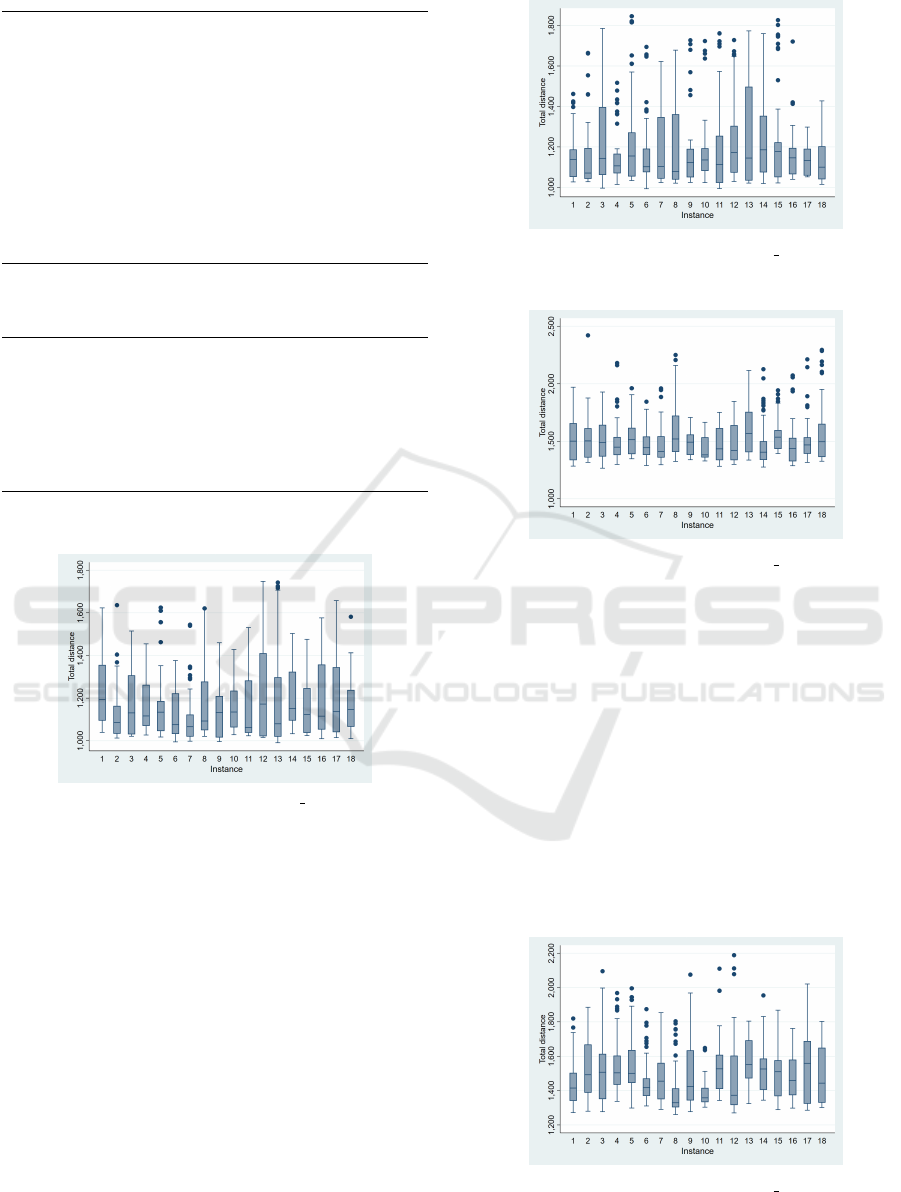
Fig. 9, Fig. 10, Fig. 11 and Fig. 12 show

the variance analysis of two benchmarks namely

Solomon 100 R108 and RC201 with ﬁxed and uni-

form recombination operator. We picked two bench-

marks belonging to two different families of bench-

marks. The box plot depicts the total distances over

18 instances. The experiment is repeated 36 times

(2x18 times) for each benchmark. The overall dis-

tribution of the total distance data and its skewness

over the instances are fairly close, which indicate that

the experiment is repeatable. Also, we can notice that

the R108 benchmark is slightly less repeatable than

the R201 benchmark. Moreover, no major difference

ECTA 2021 - 13th International Conference on Evolutionary Computation Theory and Applications

102

RC102 Sample Solution

Total Distance : 1532.44

Average Time Per Route : 196.52

Route 1 (Time= 231.32) : 0-92-50-27-29-31-34-93-94-80-0

Route 2 (Time= 219.50) : 0-83-19-23-18-48-21-25-24-0

Route 3 (Time= 237.41) : 0-39-36-40-38-41-43-35-37-72-0

Route 4 (Time= 226.72) : 0-98-73-79-7-46-4-2-100-70-0

Route 5 (Time= 235.49) : 0-33-26-28-30-32-89-0

Route 6 (Time= 228.24) : 0-65-52-99-57-86-74-77-0

Route 7 (Time= 167.06) : 0-64-22-49-20-0

Route 8 (Time= 100.24) : 0-90-0

Route 9 (Time= 133.83) : 0-42-44-61-81-0

Route 10 (Time= 175.13) : 0-85-63-76-51-84-56-66-0

Route 11 (Time= 218.26) : 0-69-88-53-78-17-13-0

Route 12 (Time= 180.00) : 0-1-3-45-5-8-6-55-68-0

Route 13 (Time= 191.93) : 0-12-14-47-16-15-9-10-60-0

Route 14 (Time= 222.19) : 0-82-11-87-59-97-75-58-0

Route 15 (Time= 180.52) : 0-91-95-62-67-71-54-96-0

Figure 7: RC102 Typical Solution.

RC202 Sample Solution

Total Distance : 1174.23

Average Time Per Route : 716.13

Route 1 (Time= 894.16) : 0-91-95-85-63-33-34-31-29-27-26-28-30-32-89-24-25-77-58-

52-0

Route 2 (Time= 929.12) : 0-69-98-88-53-99-57-86-87-9-10-59-97-75-74-13-17-60-100-

70-96-93-94-80-0

Route 3 (Time= 775.57) : 0-82-14-47-16-15-11-12-78-73-79-7-6-8-46-4-43-35-37-0

Route 4 (Time= 610.80) : 0-65-83-64-19-23-21-48-18-76-51-84-49-22-20-56-66-0

Route 5 (Time= 670.14) : 0-2-45-5-3-1-42-39-36-44-40-38-41-72-54-68-55-0

Route 6 (Time= 417.00) : 0-92-62-50-67-71-81-61-90-0

Figure 8: RC202 Typical Solution.

Figure 9: Variance analysis for Solomon 100 R108 with a

uniform recombination operator.

in the distribution and skewness is noticed between

ﬁxed and uniform recombination options.

For illustration purposes, we select the Pareto

front (one out of the 36 instances) containing the low-

est total distance point for the benchmark C201 (size

100). A typical Pareto front surface (with 3 objec-

tives) is shown in Fig. 13, where we apply a trian-

gulation to the Pareto points and plot it as a trian-

gular surface. Here in this example, the number of

routes varies between 3 and 19, the total distance be-

tween 591.56 and 3840, and the average time between

1759.43 and 3197.19. The standard deviation for to-

tal distance is 888.18, for the number of routes it is

4.06 and for the average time per route it is 281.64. In

general, we observe a positive correlation between the

number of routes and the total distance and an inverse

correlation between the number of routes and average

Figure 10: Variance analysis for Solomon 100 R108 with a

ﬁxed recombination operator.

Figure 11: Variance analysis for Solomon 100 R201 with a

uniform recombination operator.

time. The hypervolume (HV) indicator is a measure

for comparing Pareto sets in term of the closeness and

the spread of the solutions with respect to the Pareto

front. For Fig. 13, a good value of HV = 0.85 is ob-

tained given a reference point r=1.3 (30% larger than

the nadir point) (Ishibuchi et al., 2018).

Lastly, the visualization of the obtained solutions

is very helpful in presenting the ﬁnal results. Fig. 14,

Fig. 15, and Fig. 16 are sample solution depictions

of benchmark or more precisely the topological maps

(with size 100). More explicitly, C104 has a total

distance of 824.78, a number of routes equals to 10,

and an average time of 995.40. In the comparison of

Figure 12: Variance analysis for Solomon 100 R201 with a

ﬁxed recombination operator.

A Strength Pareto Evolutionary Algorithm for Solving the Capacitated Vehicle Routing Problem with Time Windows

103

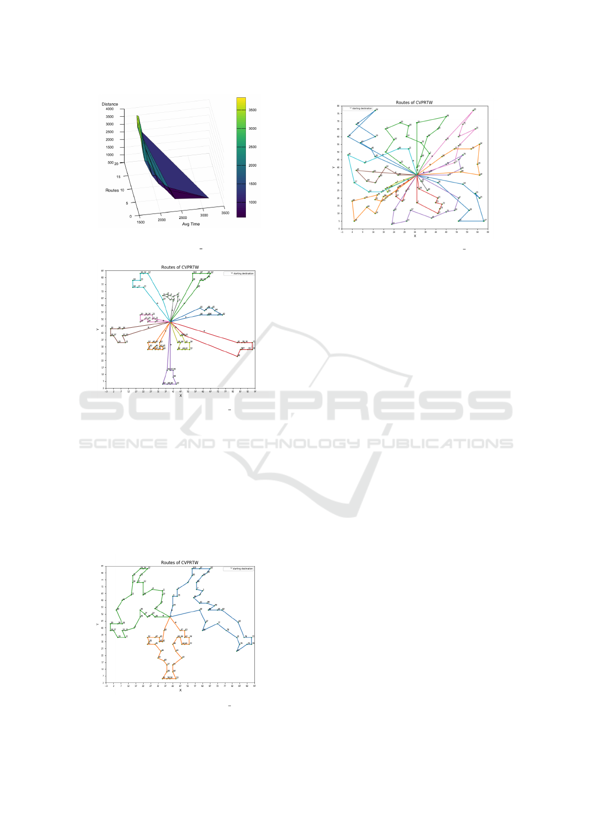
Figure 13: A visual representation sample of the Pareto

front surface obtained for Solomon 100 C201.

Figure 14: Network topology for Solomon 100 C104: dis-

tance = 824.78, routes = 10, time = 995.40.

these 3 benchmarks, C104 is situated in the middle in

terms of total distance, number of routes and average

time. C201 has the shortest total distance of 591.56,

a number of routes equals to 3, and average time of

3197.19. Clearly, in C201 we can see the reduced

number of routes and the short distance they cover

since the nodes on the routes are juxtaposed. Whereas

R103 has the highest total distance of 1240.08 which

is justiﬁable since the number of routes is elevated

and equals to 15 and it covers higher distance between

Figure 15: Network topology for Solomon 100 C201: dis-

tance = 591.56, routes = 3, time = 3197.19.

Figure 16: Network topology for Solomon 100 R103: dis-

tance = 1240.08, routes = 15, time = 196.46.

nodes on the routes. As for its average time it is equal

to 196.46. Concerning the average times, not much

can be inferred from the plots since the problem is

asymmetric but one can clearly reiterate the inverse

correlation between the number of routes and the av-

erage time.

6 CONCLUDING REMARKS

In this work, we propose a novel approach using a hy-

brid SPEA2 augmented with a hill climbing operator

to solve the CVRPTW problem optimizing for three

objectives: the total distance travelled, the number of

routes and the average time per route. The last objec-

tive is deemed necessary to reduce driver cost time

and balance the routes. Satisfactory results are re-

ported when running the widely studied Solomon’s 56

100-customer instances benchmark (a 43% improve-

ment when compared to a main stream bi-objective

BCO algorithm). In fact, considering three objec-

tives improves globally the best two standard objec-

tives since it guides the meta heuristic search toward

favorable search areas. We checked our proposed al-

gorithm for the bi-objectives case and the results do

not rebut this claim. On the other hand, the local

search is necessary to ensure quality results despite

the latency introduced. The complexity added to the

solution in order to improve quality of the solution is

in accordance with the paradox: quality results ver-

sus speed of convergence (Reimann et al., 2003). As

for the simplicity measure, the algorithm is not very

hard to conﬁgure across different type of classes for

this benchmark. Concerning the ﬂexibility of the pro-

posed algorithm, future work should examine scaling

this algorithmic solution to handle very large bench-

marks or very deploying it on different variants of

VRP such as: the green version of the CVRPTW that

ECTA 2021 - 13th International Conference on Evolutionary Computation Theory and Applications

104

accounts for carbon emissions (Lin et al., 2014), or

VRP with soft timing constraints, which if violated

we must account for a penalty. Ambitious future work

can also account for trafﬁc, i.e. higher cost routes in

city centers (Rizzoli et al., 2004) in what is known as

time dependent VRPTW. Another extension could be

to target split delivery vehicle routing problem with

time windows (SDVRPTW) where the delivery to a

customer can be split between any number of vehicles

resulting in considerable improvements in terms num-

ber of vehicles used and cost (Da Silva et al., 2014;

Feillet et al., 2006).

On the other hand, this work can be generalized to

address a different class of VRP altogether, namely

the VRP with backhauls (VRPB) (Toth and Vigo,

2001). Lastly, it is also interesting for future work

to add problem knowledge to the reproduction oper-

ators such as the one proposed in (Hsu and Chiang,

2012).

ACKNOWLEDGEMENTS

We thank dearly Dr. Janka Chlebikova and Dr. Mo-

hamad Bader-El-Den from the School of Computing

at University of Portsmouth for their valuable support.

Numerical computations were done on the Sciama

High Performance Compute (HPC) cluster which is

supported by the ICG, SEPNet and the University of

Portsmouth.

REFERENCES

Bychkov, I. and Batsyn, M. (2018). A hybrid approach

for the capacitated vehicle routing problem with time

windows. In OPTA-SCL. CEUR Workshop Proceed-

ings.

Chiang, T.-C. and Hsu, W.-H. (2014). A knowledge-based

evolutionary algorithm for the multiobjective vehicle

routing problem with time windows. Computers &

Operations Research, 45:25–37.

Czech, Z. J. and Czarnas, P. (2002). Parallel simulated

annealing for the vehicle routing problem with time

windows. In Proceedings 10th Euromicro workshop

on parallel, distributed and network-based process-

ing, pages 376–383. IEEE.

Da Silva, M. D. M., Subramanian, A., and Ochi, L. S.

(2014). An iterated local search heuristic for the split

delivery vehicle routing problem. In ROADEF-15

eme

congr

es annuel de la Soci

e franc¸aise de recherche

erationnelle et d’aide

a la d

ecision.

Dash, M. and Anekal, B. I. (2014). Variables reduction in

vehicle routing problems. SPC ERA IJBM, 2(6).

Dixit, A., Mishra, A., and Shukla, A. (2019). Vehicle rout-

ing problem with time windows using meta-heuristic

algorithms: a survey. In Harmony search and na-

ture inspired optimization algorithms, pages 539–546.

Springer.

Feillet, D., Dejax, P., Gendreau, M., and Gueguen, C.

(2006). Vehicle routing with time windows and split

deliveries. Technical Paper, 851.

Garcia-Najera, A. and Bullinaria, J. A. (2011). An im-

proved multi-objective evolutionary algorithm for the

vehicle routing problem with time windows. Comput-

ers & Operations Research, 38(1):287–300.

Hsu, W.-H. and Chiang, T.-C. (2012). A multiobjective evo-

lutionary algorithm with enhanced reproduction oper-

ators for the vehicle routing problem with time win-

dows. In 2012 IEEE Congress on Evolutionary Com-

putation, pages 1–8. IEEE.

Ishibuchi, H., Imada, R., Setoguchi, Y., and Nojima, Y.

(2018). How to specify a reference point in hyper-

volume calculation for fair performance comparison.

Evolutionary computation, 26(3):411–440.

Jawarneh, S. and Abdullah, S. (2015). Sequential insertion

heuristic with adaptive bee colony optimisation algo-

rithm for vehicle routing problem with time windows.

PloS one, 10(7):e0130224.

King, R. A., Deb, K., and Rughooputh, H. (2010). Compar-

ison of nsga-ii and spea2 on the multiobjective envi-

ronmental/economic dispatch problem. University of

Mauritius Research Journal, 16(1):485–511.

Li, W., Dai, H., and Zhang, D. (2015). The relationship

between maximum completion time and total comple-

tion time in ﬂowshop production. Procedia Manufac-

turing, 1:146–156.

Lin, C., Choy, K. L., Ho, G. T., Chung, S. H., and Lam, H.

(2014). Survey of green vehicle routing problem: past

and future trends. Expert systems with applications,

41(4):1118–1138.

Luke, S. (2013). Essentials of metaheuristics. lulu, 2013.

Metaheuristics in large-scale global continues op-

timization: A survey, available at: http://cs. gmu.

edu/ sean/book/metaheuristics.

Marrouche, W., Farah, R., and Harmanani, H. M. (2018).

A strength pareto evolutionary algorithm for optimiz-

ing system-on-chip test schedules. International Jour-

nal of Computational Intelligence and Applications,

17(02):1850010.

Meryem, B. and Abdelmadjid, B. (2015). Resolving a ve-

hicle routing problem with heterogeneous ﬂeet, mixed

backhauls and time windows using cuckoo behaviour

approach. International Journal of Operational Re-

search, 24(2):132–144.

Messaoud, E., El Idrissi, A. E. B., and Alaoui, A. E. (2018).

The green dynamic vehicle routing problem in sus-

tainable transport. In 2018 4th International Con-

ference on Logistics Operations Management (GOL),

pages 1–6. IEEE.

Minocha, B., Tripathi, S., and Mohan, C. (2011). Solving

vehicle routing and scheduling problems using hybrid

genetic algorithm. In 2011 3rd international confer-

ence on electronics computer technology, volume 2,

pages 189–193. Ieee.

A Strength Pareto Evolutionary Algorithm for Solving the Capacitated Vehicle Routing Problem with Time Windows

105

Reimann, M., Doerner, K., and Hartl, R. F. (2003). Ana-

lyzing a uniﬁed ant system for the vrp and some of its

variants. In Workshops on Applications of Evolution-

ary Computation, pages 300–310. Springer.

Rizzoli, A. E., Oliverio, F., Montemanni, R., and Gam-

bardella, L. M. (2004). Ant colony optimisation for

vehicle routing problems: from theory to applications.

Galleria Rassegna Bimestrale Di Cultura, 9(1):1–50.

Taha, A., Hachimi, M., and Moudden, A. (2017). A dis-

crete bat algorithm for the vehicle routing problem

with time windows. In 2017 International Colloquium

on Logistics and Supply Chain Management (LOGIS-

TIQUA), pages 65–70. IEEE.

Tan, K. C., Chew, Y. H., and Lee, L. H. (2006). A hybrid

multiobjective evolutionary algorithm for solving ve-

hicle routing problem with time windows. Computa-

tional Optimization and Applications, 34(1):115–151.

Toth, P. and Vigo, D. (2001). The vehicle routing problem:

Society for industrial and applied mathematics. Siam

Monographs on Discrete Mathematics and Applica-

tions.

Udin, K., Gui, R., and Rahmawan, A. (2017). Green ve-

hicle routing problem with heterogeneous ﬂeet and

time windows. In Proceedings of the 6th International

Conference on Software and Computer Applications,

pages 223–227.

Vidal, T., Crainic, T. G., Gendreau, M., Lahrichi, N., and

Rei, W. (2012). A hybrid genetic algorithm for multi-

depot and periodic vehicle routing problems. Opera-

tions Research, 60(3):611–624.

Xiao, L., Hajjam-El-Hassani, A., and Dridi, M. (2017). An

application of extended cuckoo search to vehicle rout-

ing problem. In 2017 International Colloquium on

Logistics and Supply Chain Management (LOGISTI-

QUA), pages 31–35. IEEE.

Yasin, M. and Vincent, F. Y. (2013). A simulated anneal-

ing heuristic for the green vehicle routing problem.

In Proceedings of the institute of industrial engineers

Asian conference 2013, pages 1261–1269. Springer.

Zitzler, E. (2001). Spea2: Improving the performance of the

strength pareto evolutionary algorithm. Computer En-

gineering and Communication Networks Lab (TIK).

Zitzler, E., Laumanns, M., and Bleuler, S. (2004). A tutorial

on evolutionary multiobjective optimization. Meta-

heuristics for multiobjective optimisation, pages 3–37.

ECTA 2021 - 13th International Conference on Evolutionary Computation Theory and Applications

106