Multiobjective Bimatrix Game with Fuzzy Payoffs and Its Solution
Method using Necessity Measure and Weighted Tchebycheff Norm
Hitoshi Yano
1 a
and Ichiro Nishizaki
2 b
1
Graduate School of Humanities and Social Sciences, Nagoya City University, Nagoya, 467-8501, Japan
2
Graduate School of Advanced Science and Engineering, Hiroshima University, Higashi-Hiroshima, 739-8527, Japan
Keywords:
Bimatrix Games with Fuzzy Payoffs, Multiobjective Programming, Necessity Measure, Interactive Method,
Weighted Tchebycheff Norm Method.
Abstract:
In this paper, we propose an interactive algorithm for multiobjective bimatrix games with fuzzy payoffs. Us-
ing necessity measure and the weighted Tchebycheff norm method, an equilibrium solution concept is de-
fined, which depends on weighting vectors specified by each player. Since it is very difficult to obtain such
equilibrium solutions directly, instead of equilibrium conditions in the necessity measure space, equilibrium
conditions in the expected payoff space are provided. Under the assumption that a player can estimate the op-
ponent player’s preference as the weighting vector of the weighted Tchebycheff norm method, the interactive
algorithm is proposed to obtain a satisfactory solution of the player from among an equilibrium solution set
by updating the weighting vector.
1 INTRODUCTION
Recently, various types of noncooperative games un-
der uncertainty in strategic form have been inves-
tigated, and the corresponding equilibrium solution
concepts have been proposed (Larbani, 2009). Cam-
pos (Campos, 1989) first formulated two-person zero-
sum games with fuzzy payoffs. In her method, un-
der the assumption that each element of a fuzzy pay-
off matrix is defined as a triangular fuzzy number
(Dubois and Prade, 1980), such games are reduced
to two kinds of linear programming problems by us-
ing Yager’s method (Yager, 1981). Similarly, Li (Li,
1999) formulated two-person zero-sum games with
triangular fuzzy numbers as two kinds of multiobjec-
tive programming problems, in which each objective
function is corresponding to the extreme point of a
triangular fuzzy number. Bector et al. (Bector et al.,
2004) also formulated two-person zero-sum games
with fuzzy payoffs as two kinds of optimization prob-
lems which depends on the defuzzification functions
(Yager, 1981). Moreover, using the threshold values
for the level sets (Dubois and Prade, 1980) and the
ordering relation called the fuzzy max order, Maeda
(Maeda, 2003) reduced two-person zero-sum games
a
https://orcid.org/0000-0002-4818-5695
b
https://orcid.org/0000-0002-0060-4360
with triangular fuzzy numbers to two kinds of linear
programming problems.
On the other hand, to deal with bimatrix games
with triangular fuzzy numbers, Maeda (Maeda, 2000)
defined an equilibrium solution concept using possi-
bility measure and the threshold values for the level
sets (Dubois and Prade, 1980). He formulated the cor-
responding mathematical programming problem to
obtain such parametric equilibrium solutions. Mako
et al. (Mak
´
o and Salamon, 2020) focused on bi-
matrix games with LR fuzzy numbers. Correspond-
ing to the fuzzy Nash-equilibrium solution concept,
they proposed the fuzzy correlated equilibrium so-
lution concept, which is based on a joint distribu-
tion for mixed strategies of both players. Gao (Gao,
2013) introduced three kinds of uncertain equilibrium
solution concepts based on uncertainty theory (Liu,
2007), which depend on the values of confidence lev-
els. From a similar point of view based on uncertainty
theory, Tang et al. (Tang and Li, 2020) proposed an
uncertain equilibrium solution concept based on the
Hurwicz criterion.
For multiobjective bimatrix games, Corley (Cor-
ley, 1985) first defined a Pareto equilibrium so-
lution concept, and formulated quadratic program-
ming problems to obtain Pareto equilibrium solu-
tions through the Karush-Kuhn-Tucker conditions, in
which multiobjective functions are scalarized by the
Yano, H. and Nishizaki, I.
Multiobjective Bimatrix Game with Fuzzy Payoffs and Its Solution Method using Necessity Measure and Weighted Tchebycheff Norm.
DOI: 10.5220/0010630700003063
In Proceedings of the 13th International Joint Conference on Computational Intelligence (IJCCI 2021), pages 159-166
ISBN: 978-989-758-534-0; ISSN: 2184-3236
Copyright © 2023 by SCITEPRESS – Science and Technology Publications, Lda. Under CC license (CC BY-NC-ND 4.0)
159

weighting coefficients. Nishizaki et al. (Nishizaki
and Sakawa, 1995) formulated multiobjective bima-
trix games incorporating fuzzy goals. They trans-
formed multiobjective bimatrix games into usual bi-
matrix games by applying the weighting methods
or the minimum operator (Sakawa, 1993), and de-
fined the corresponding equilibrium solution con-
cepts. They formulated the nonlinear programming
problems to obtain such equilibrium solutions. Us-
ing dominance cones proposed by Yu (Yu, 1985),
Nishizaki et al. (Nishizaki and Notsu, 2007) defined
a nondominated equilibrium solution concept which
is a generalization of Nash equilibrium solution con-
cept, and formulate nonlinear programming problem
to obtain nondominated equilibrium solutions by ap-
plying the Tamura and Miura conditions (Tamura and
Miura, 1979).
In such a situation, in this paper, we propose an in-
teractive algorithm for multiobjective bimatrix games
with fuzzy payoffs. Using necessity measure (Dubois
and Prade, 1980) and the weighted Tchebycheff norm
method (Bowman, 1976), an equilibrium solution
concept is introduced, which depends on weighting
vectors of both players. To obtain such equilibrium
solutions, the relationships between the equilibrium
conditions in the membership function space and the
equilibrium conditions in the expected payoff space.
Under the assumption that a player can estimate the
opponent player’s weighting vector, the interactive al-
gorithm is proposed to obtain a satisfactory solution
of the player from among an equilibrium solution set
by updating the weighting vector.
In section 2, we propose an interactive decision
making method for multiobjective bimatrix games
with fuzzy payoffs. Using necessity measure and the
weighted Tchebycheff norm method, an equilibrium
solution concept is introduced. An interactive algo-
rithm is developed to obtain a satisfactory solution of
a player from among a equilibrium solution set by up-
dating the weighting vector. In section 3, a numerical
example of two-objectve bimatrix games with fuzzy
payoffs illustrates interactive processes under a hypo-
thetical player to show the efficiency of the proposed
method.
2 MULTIOBJECTIVE BIMATRIX
GAMES WITH FUZZY
PAYOFFS
In this section, we consider multiobjective bimatrix
games with fuzzy payoffs. Let i ∈ {1,2,·· · , m} be
a pure strategy of Player 1 and j ∈ {1,2,··· ,n} be a
pure strategy of Player 2.
˜
A
k
= ( ˜a
ki j
),k = 1,...,K
are Player 1’s (m × n)-payoff matrices, and
˜
B
l
=
(
˜
b
li j
),l = 1,· ·· , L are Player 2’s (m × n)-payoff ma-
trices. Elements ˜a
ki j
and
˜
b
li j
are LR fuzzy numbers
(Dubois and Prade, 1980) whose membership func-
tions are defined as follows.
µ
e
a
ki j
(s) =



L
1

a
ki j
−s
α
ki j

a
ki j
− α
ki j
≤ s ≤ a
ki j
R
1

s−a
ki j
β
ki j

a
ki j
≤ s ≤ a
ki j
+ β
ki j
µ
e
b
li j
(t) =



L
2

b
li j
−t
γ
li j

b
li j
− γ
li j
≤ t ≤ b
li j
R
2

t−b
li j
δ
li j

b
li j
≤ t ≤ b
li j
+ δ
li j
where L
1
(·) is a type function (Dubois and Prade,
1980) which is strictly monotone decreasing on the
interval [0,1], and L
1
(0) = 1, L
1
(1) = 0. For the other
type functions R
1
(·),L
2
(·) and R
2
(·), similar condi-
tions are satisfied. In the following, LR fuzzy num-
bers ˜a
ki j
and
˜
b
li j
are denoted as (a
ki j
,α
ki j
,β
ki j
)
LR
and
(b
li j
,γ
li j
,δ
li j
)
LR
, respectively. Let
X
def
= {x ∈ R
m
|
m
∑
i=1
x
i
= 1, x
i
≥ 0, i = 1,·· · ,m}
Y
def
= {y ∈ R
n
|
n
∑
j=1
y
j
= 1, y
j
≥ 0, j = 1,·· · ,n}
be sets of mixed strategies for Players 1 and 2. Then,
a multiobjective bimatrix game with fuzzy payoffs is
formally expressed as follows.
P1
maximize
x∈X
(x
T
˜
A
1
y,.. .,x
T
˜
A
K
y) (1a)
maximize
y∈Y
(x
T
˜
B
1
y,.. .,x
T
˜
B
L
y) (1b)
It should be noted here that fuzzy expected payoffs
x
T
˜
A
k
y,k = 1,· ·· ,K and x
T
˜
B
l
y,l = 1,· ·· , L are ex-
pressed as LR fuzzy numbers because of the property
(Dubois and Prade, 1980) of LR fuzzy numbers.
In P1, it is assumed that Players 1 and 2 have fuzzy
goals
˜
G
1k
,k = 1, ··· ,K,
˜
G
2l
,l = 1, ·· · ,L for their ex-
pected payoffs, and the corresponding membership
functions µ
˜
G
1k
(s),k = 1,· ·· , K, µ
˜
G
2l
(t),l = 1,·· · ,L
are linear or nonlinear functions, which are continu-
ous and strictly increasing on the corresponding sup-
port for LR fuzzy numbers x
T
˜
A
k
y or x
T
˜
B
l
y, i.e.,
S
def
= {s ∈ R
1
| µ
x
T
˜
A
k
y
(s) > 0}, (2)
T
def
= {t ∈ R
1
| µ
x
T
˜
B
l
y
(t) > 0}. (3)
To deal with fuzzy expected payoffs x
T
˜
A
k
y and
x
T
˜
B
l
y, we introduce concepts of the possibility mea-
sure and the necessity measure (Dubois and Prade,
FCTA 2021 - 13th International Conference on Fuzzy Computation Theory and Applications
160

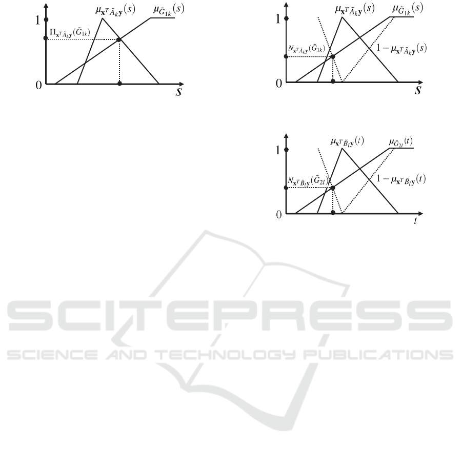
Figure 1: The possibility measure Π
x
T
˜
A
k
y
(
˜
G
1k
).
1980). A possibility degree that fuzzy expected pay-
offs x
T
˜
A
k
y attains the fuzzy goal
˜
G
1k
can be expressed
by using a possibility measure defined as follows.
Π
x
T
˜
A
k
y
(
˜
G
1k
)
def
= sup
s
min(µ
x
T
˜
A
k
y
(s),µ
˜
G
1k
(s))
Fig.1 shows the relationship between the possibil-
ity measure Π
x
T
˜
A
k
y
(
˜
G
1k
) and the membership func-
tions µ
x
T
˜
A
k
y
(u) and µ
˜
G
1k
(u). Based on the possibil-
ity measure, the following necessity measure (Dubois
and Prade, 1980) is defined as a non-possibility de-
gree that the “complement” of fuzzy expected payoffs
x
T
˜
A
k
y attains the fuzzy goal
˜
G
1k
.
N
x
T
˜
A
k
y
(
˜
G
1k
)
def
= inf
s
max(1 − µ
x
T
˜
A
k
y
(s),µ
˜
G
1k
(s))
Dubois and Prade (1980) interpreted the above func-
tion as a necessity measure by analogy with modal
logic where “a subset C is necessary” is equivalent to
“non-C is not possible”. Fig.2 shows the relationship
between the necessity measure N
x
T
˜
A
k
y
(
˜
G
1k
) and the
membership functions µ
x
T
˜
A
k
y
(u) and µ
˜
G
1k
(u).
In this paper, we adopt the above mentioned ne-
cessity measure to deal with fuzzy expected payoffs.
Then, P1 can be interpreted as the following problem.
P2
maximize
x∈X

N
x
T
˜
A
1
y
(
˜
G
11
),.. .,N
x
T
˜
A
K
y
(
˜
G
1K
)

(4a)
maximize
y∈Y

N
x
T
˜
B
1
y
(
˜
G
21
),.. .,N
x
T
˜
B
L
y
(
˜
G
2L
)

, (4b)
where the necessity measures are defined as follows (
see Fig.2 and Fig.3).
N
x
T
˜
A
k
y
(
˜
G
1k
)
def
= inf
s
max

1 − µ
x
T
˜
A
k
y
(s),µ
˜
G
1k
(s)

,
k = 1,.. .,K (5)
N
x
T
˜
B
l
y
(
˜
G
2l
)
def
= inf
t
max

1 − µ
x
T
˜
B
l
y
(t),µ
˜
G
2l
(t)

,
l = 1, ..., L (6)
From the assumption of the membership functions
µ
˜
G
1k
(s),k = 1,... ,K, µ
˜
G
2l
(t),l = 1,. .. ,L, the follow-
ing relations always hold.
0 < N
x
T
˜
A
k
y
(
˜
G
1k
) < 1, k = 1,. ..,K,∀x ∈ X,∀y ∈ Y
0 < N
x
T
˜
B
l
y
(
˜
G
2l
) < 1, l = 1,.. .,L,∀x ∈ X,∀y ∈ Y
Figure 2: The necessity measure N
x
T
˜
A
k
y
(
˜
G
1k
).
Figure 3: The necessity measure N
x
T
˜
B
l
y
(
˜
G
2l
).
By applying the weighted Tchebycheff norm
method, P2 can be transformed into a bimatrix game
defined as follows.
P3(w
1
,w
2
)
maximize
x∈X
min
k=1,...,K
N
x
T
˜
A
k
y
(
˜
G
1k
)/w
1k
(7a)
maximize
y∈Y
min
l=1,...,L
N
x
T
˜
B
l
y
(
˜
G
2l
)/w
2l
(7b)
where w
1
def
= (w
11
,·· · , w
1K
) ∈ W
1
and w
2
def
=
(w
21
,·· · , w
2L
) ∈ W
2
are the weighting vectors for the
necessity measures, and
W
1
def
= {w
1
∈ R
K
|
K
∑
k=1
w
1k
= 1,w
1k
> 0,k = 1, · · · ,K},
W
2
def
= {w
2
∈ R
L
|
L
∑
l=1
w
2l
= 1,w
2l
> 0,l = 1,··· ,L}.
Now, we can introduce an equilibrium solution con-
cept for P3(w
1
,w
2
), which depends on the weighting
vectors.
Definition 1. (x
∗
,y
∗
) is an equilibrium solution to
P3(w
1
,w
2
),if the following inequalities hold.
min
k=1,...,K
N
x
∗T
˜
A
k
y
∗
(
˜
G
1k
)/w
1k
≥ min
k=1,...,K
N
x
T
˜
A
k
y
∗
(
˜
G
1k
)/w
1k
, ∀x ∈ X (8a)
min
l=1,...,L
N
x
∗T
˜
B
l
y
∗
(
˜
G
2l
)/w
2l
≥ min
l=1,...,L
N
x
∗T
˜
B
l
y
(
˜
G
2l
)/w
2l
, ∀y ∈ Y (8b)
It is very difficult to obtain the equilibrium so-
lution to P3(w
1
,w
2
) from the computational aspect,
Multiobjective Bimatrix Game with Fuzzy Payoffs and Its Solution Method using Necessity Measure and Weighted Tchebycheff Norm
161

because of the definition (5), (6), and the non-
linear membership functions µ
˜
G
1k
(s),k = 1,.. .,K,
µ
˜
G
2l
(t),l = 1, ·· · ,L. To circumvent such a difficulty,
at first, we consider the following bimatrix game,
which is equivalent to P3(w
1
,w
2
).
P4(w
1
,w
2
)
maximize
x∈X, v
1
∈R
1
v
1
subject to
N
x
T
˜
A
k
y
(
˜
G
1k
)/w
1k
≥ v
1
, k = 1, .. .,K (9a)
maximize
y∈Y, v
2
∈R
1
v
2
subject to
N
x
T
˜
B
l
y
(
˜
G
2l
)/w
2l
≥ v
2
, l = 1, ..., L (9b)
Let (x
∗
,y
∗
,v
∗
1
,v
∗
2
) be an equilibrium solution to
P4(w
1
,w
2
). Then, the following equalities hold at
(x
∗
,y
∗
,v
∗
1
,v
∗
2
).
min
k=1,...,K

N
x
∗T
˜
A
k
y
∗
(
˜
G
1k
)/w
1k

= v
∗
1
(10a)
min
l=1,...,L

N
x
∗T
˜
B
l
y
∗
(
˜
G
2l
)/w
2l

= v
∗
2
(10b)
We denote α-level sets for LR fuzzy numbers x
∗T
˜
A
k
y
∗
and x
∗T
˜
B
l
y
∗
as the closed intervals :
(x
∗T
˜
A
k
y
∗
)
α
def
= [x
∗T
A
L
k, α
y
∗
,x
∗T
A
R
k, α
y
∗
],
(x
∗T
˜
B
l
y
∗
)
α
def
= [x
∗T
B
L
l,α
y
∗
,x
∗T
B
R
l,α
y
∗
],
respectively, where A
L
k, α
def
= (a
L
ki j,α
), A
R
k, α
def
= (a
R
ki j,α
),
B
L
l,α
def
= (b
L
li j,α
) B
R
l,α
def
= (b
R
li j,α
) are (m × n)-matrices.
a
L
ki j,α
and a
R
li j,α
mean the left and the right hand side
extreme points of the α-level set for ˜a
ki j
. Similarly,
b
L
ki j,α
and b
R
li j,α
mean the extreme points of the α-
level set for
˜
b
ki j
.
Now, let us focus on the equality (10a). We
denote the left hand side of the membership func-
tion µ
x
∗T
˜
A
k
y
∗
(s) as µ
L
x
∗T
˜
A
k
y
∗
(s). Since the member-
ship function µ
˜
G
1k
(s) is strictly monotone increas-
ing with respect to s ∈ S, the equality (10a) means
that 1 − µ
L
x
∗T
˜
A
k
y
∗
(s) ≥ w
1k
v
∗
1
, µ
˜
G
1k
(s) ≥ w
1k
v
∗
1
. Since
µ
L
x
∗T
˜
A
k
y
∗
(s) is strictly monotone increasing with re-
spect to s ∈ S, it holds that (µ
L
x
∗T
˜
A
k
y
∗
)
−1
(1−w
1k
v
∗
1
) ≥ s
and µ
−1
˜
G
1k
(w
1k
v
∗
1
) ≤ s. As a result, we can obtain the
following inequalities.
(µ
L
x
∗T
˜
A
k
y
∗
)
−1
(1 − w
1k
v
∗
1
) ≥ µ
−1
˜
G
1k
(w
1k
v
∗
1
),k = 1, ··· ,K
It should be noted here that, from the property of
the LR fuzzy number x
∗T
˜
A
k
y
∗
, we can express the
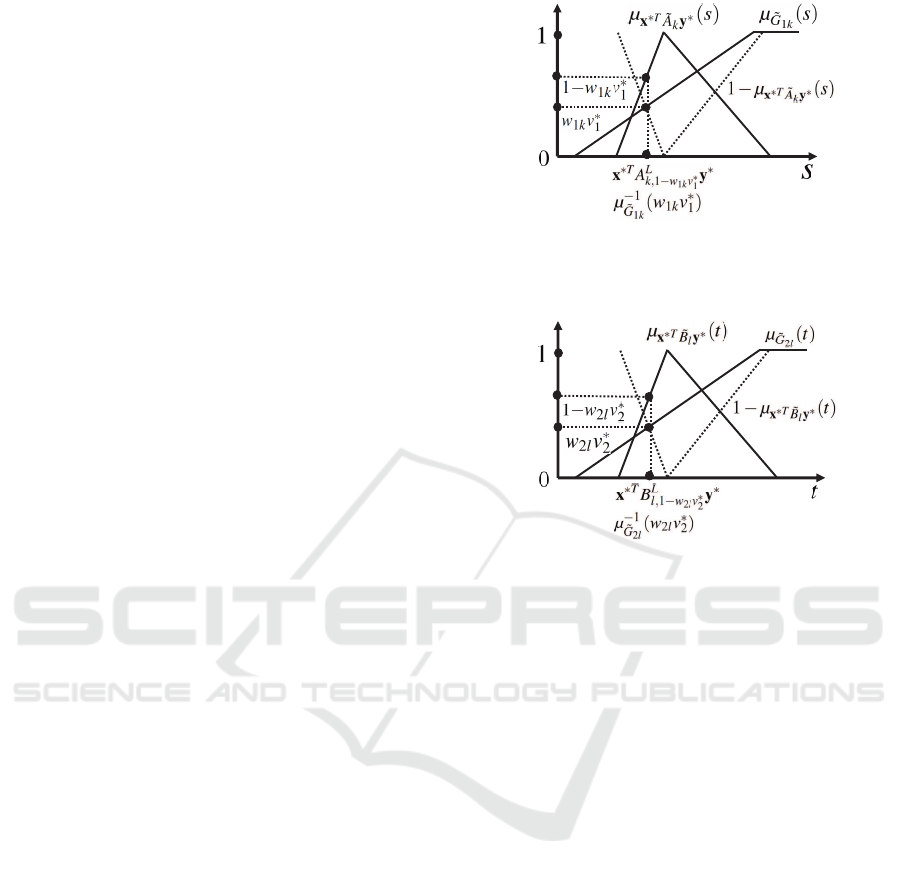
Figure 4: The relationship between N
x
∗T
˜
A
k
y
∗
(
˜
G
1k
) and
x
∗T
A
L
k, 1−w
1k
v
∗
1
y
∗
− µ
−1
˜
G
1k
(w
1k
v
∗
1
) = 0.
Figure 5: The relationship between N
x
∗T
˜
B
l
y
∗
(
˜
G
2l
) and
x
∗T
B
L
l,1−w
2l
v
∗
2
y
∗
− µ
−1
˜
G
2l
(w
2l
v
∗
2
) = 0.
above inequalities as follows, where A
L
k, 1−w
1k
v
∗
1
def
=
(a
L
ki j,1−w
1k
v
∗
1
).
x
∗T
A
L
k, 1−w
1k
v
∗
1
y
∗
≥ µ
−1
˜
G
1k
(w
1k
v
∗
1
),k = 1, ··· ,K
Similarly, from the equality (10b), we can ob-
tain the following inequalities, where B
L
l,1−w
2l
v
∗
2
def
=
(b
L
li j,1−w
2l
v
∗
2
).
x
∗T
B
L
l,1−w
2l
v
∗
2
y
∗
≥ µ
−1
˜
G
2l
(w
2l
v
∗
2
),l = 1,·· · , L
From such a point of view, the equalities (10a) and
(10b) are equivalent to the following ones (see Fig.4
and Fig.5).
min
k=1,...,K

x
∗T
A
L
k, 1−w
1k
v
∗
1
y
∗
− µ
−1
˜
G
1k
(w
1k
v
∗
1
)

= 0
(11a)
min
l=1,...,L

x
∗T
B
L
l,1−w
2l
v
∗
2
y
∗
− µ
−1
˜
G
2l
(w
2l
v
∗
2
)

= 0 (11b)
Corresponding to (11a) and (11b), we consider the
following bimatrix game, in which not only (w
1
,w
2
)
but also (v
∗
1
,v
∗
2
) are given as parameters.
P5(w
1
,w
2
;v
∗
1
,v
∗
2
)
maximize
x∈X
min
k=1,...,K
{x
T
A
L
k, 1−w
1k
v
∗
1
y − µ
−1
˜
G
1k
(w
1k
v
∗
1
)}
maximize
y∈Y
min
l=1,...,L
{x
T
B
L
l,1−w
2l
v
∗
2
y − µ
−1
˜
G
2l
(w
2l
v
∗
2
)}
FCTA 2021 - 13th International Conference on Fuzzy Computation Theory and Applications
162

For P5(w
1
,w
2
;v
∗
1
,v
∗
2
), we introduce an equilibrium
solution concept.
Definition 2. (x
∗
,y
∗
) is an equilibrium solution to
P5(w
1
,w
2
;v
∗
1
,v
∗
2
), if the following inequalities hold.
min
k=1,...,K
{x
∗T
A
L
k, 1−w
1k
v
∗
1
y
∗
− µ
−1
˜
G
1k
(w
1k
v
∗
1
)}
≥ min
k=1,...,K
{x
T
A
L
k, 1−w
1k
v
∗
1
y
∗
− µ
−1
˜
G
1k
(w
1k
v
∗
1
)}, ∀x ∈ X
min
l=1,...,L
{x
∗T
B
L
l,1−w
2l
v
∗
2
y
∗
− µ
−1
˜
G
2l
(w
2l
v
∗
2
)}
≥ min
l=1,...,L
{x
∗T
B
L
l,1−w
2l
v
∗
2
y − µ
−1
˜
G
2l
(w
2l
v
∗
2
)}, ∀y ∈ Y
Then, the following relationships between equi-
librium solutions to P5(w
1
,w
2
;v
∗
1
,v
∗
2
) and equilibrium
solutions to P4(w
1
,w
2
) hold.
Theorem 1. If (x
∗
,y
∗
,v
∗
1
,v
∗
2
) is an equilibrium solu-
tion to P4(w
1
,w
2
), then (x
∗
,y
∗
) is an equilibrium so-
lution to P5(w
1
,w
2
;v
∗
1
,v
∗
2
).
(Proof) : Assume that (x
∗
,y
∗
) is not an equilib-
rium solution to P5(w
1
,w
2
;v
∗
1
,v
∗
2
). Then, there exists
some x ∈ X such that
min
k=1,...,K
n
x
∗T
A
L
k,1−w
1k
v
∗
1
y
∗
− µ
−1
˜
G
1k
(w
1k
v
∗
1
)
o
<
min
k=1,...,K
n
x
T
A
L
k,1−w
1k
v
∗
1
y
∗
− µ
−1
˜
G
1k
(w
1k
v
∗
1
)
o
, (14)
or, there exists some y ∈ Y such that
min
l=1,...,L
n
x
∗T
B
L
l,1−w
2l
v
∗
2
y
∗
− µ
−1
˜
G
2l
(w
2l
v
∗
2
)
o
<
min
l=1,...,L
n
x
∗T
B
L
l,1−w
2l
v
∗
2
y − µ
−1
˜
G
2l
(w
2l
v
∗
2
)
o
. (15)
Assume that there exists some x ∈ X such that the in-
equality (14) is satisfied. Then, from (11a), the fol-
lowing relation holds.
0 = min
k=1,···,K

x
∗T
A
L
k,1−w
1k
v
∗
1
y
∗
− µ
−1
˜
G
1k
(w
1k
v
∗
1
)

< min
k=1,···,K

x
T
A
L
k,1−w
1k
v
∗
1
y
∗
− µ
−1
˜
G
1k
(w
1k
v
∗
1
)

Since (11a) is equivalent to (10a), the above relation
is equivalent to the following inequality.
v
∗
1
= min
k=1,···,K

N
x
∗T
˜
A
k
y
∗
(
˜
G
1k
)/w
1k

< min
k=1,···,K

N
x
T
˜
A
k
y
∗
(
˜
G
1k
)/w
1k

.
This contradicts the fact that (x
∗
,y
∗
,v
∗
1
,v
∗
2
) is an equi-
librium solution to P4(w
1
,w
2
). Similarly, we can
prove for the case that there exists y ∈ Y such that
(15) is satisfied.
Theorem 2. If (x
∗
,y
∗
) is an equilibrium solution to
P5(w
1
,w
2
;v
∗
1
,v
∗
2
), where the following relations hold,
min
k=1,···,K

x
∗T
A
L
k,1−w
1k
v
∗
1
y
∗
− µ
−1
˜
G
1k
(w
1k
v
∗
1
)

= 0, (16)
min
l=1,···,L

x
∗T
B
L
l,1−w
2l
v
∗
2
y
∗
− µ
−1
˜
G
2l
(w
2l
v
∗
2
)

= 0, (17)
then, (x
∗
,y
∗
,v
∗
1
,v
∗
2
) is an equilibrium solution to
P4(w
1
,w
2
).
(Proof) : Assume that (x
∗
,y
∗
,v
∗
1
,v
∗
2
) is not an
equilibrium solution to P4(w
1
,w
2
). Then, there ex-
ists some x ∈ X such that
min
k=1,...,K
N
x
∗T
˜
A
k
y
∗
(
˜
G
1k
)/w
1k
< min
k=1,...,K
N
x
T
˜
A
k
y
∗
(
˜
G
1k
)/w
1k
, (18)
or, there exists some y ∈ Y such that
min
l=1,...,L
N
x
∗T
˜
B
l
y
∗
(
˜
G
2l
)/w
2l
< min
l=1,...,L
N
x
∗T
˜
B
l
y
(
˜
G
2l
)/w
2l
. (19)
Assume that there exists some x ∈ X such that (18) is
satisfied. Then, from (16), it holds that
v
∗
1
= min
k=1,...,K

N
x
∗T
˜
A
k
y
∗
(
˜
G
1k
)/w
1k

< min
k=1,...,K

N
x
T
˜
A
k
y
∗
(
˜
G
1k
)/w
1k

.
Since (10a) is equivalent to (11a), the following rela-
tion holds.
0 = min
k=1,···,K

x
∗T
A
L
k,1−w
1k
v
∗
1
y
∗
− µ
−1
˜
G
1k
(w
1k
v
∗
1
)

< min
k=1,···,K

x
T
A
L
k,1−w
1k
v
∗
1
y
∗
− µ
−1
˜
G
1k
(w
1k
v
∗
1
)

This contradicts the fact that (x
∗
,y
∗
) is an equilibrium
solution to P5(w
1
,w
2
;v
∗
1
,v
∗
2
). Similarly, we can prove
for the case that there exists y ∈ Y such that (19) is
satisfied.
From the above theorems, instead of solving
P4(w
1
,w
2
) directly, we can obtain an equilibrium
solution to P4(w
1
,w
2
) by solving P5(w
1
,w
2
;v
∗
1
,v
∗
2
),
where (v
∗
1
,v
∗
2
) satisfies the equality conditions (16)
and (17). On the other hand, an equilibrium solution
to P5(w
1
,w
2
;v
∗
1
,v
∗
2
) is obtained by solving the follow-
ing nonlinear programming problem (Nishizaki and
Sakawa, 1995).
Multiobjective Bimatrix Game with Fuzzy Payoffs and Its Solution Method using Necessity Measure and Weighted Tchebycheff Norm
163

P6(w
1
,w
2
;v
∗
1
,v
∗
2
)
maximize
x∈X, y∈Y, p, q, σ
1
, σ
2
σ
1
+ σ
2
− p − q
subject to
A
L
k, 1−w
1k
v
∗
1
y − µ
−1
˜
G
1k
(w
1k
v
∗
1
)e
1
≤ pe
1
, k = 1, .. .,K
(20a)
x
T
B
L
l,1−w
2l
v
∗
2
− µ
−1
˜
G
2l
(w
2l
v
∗
2
)e
2
≤ qe
2
, l = 1, ..., L
(20b)
x
T
A
L
k, 1−w
1k
v
∗
1
y − µ
−1
˜
G
1k
(w
1k
v
∗
1
) ≥ σ
1
, k = 1, .. .,K
(20c)
x
T
B
L
l,1−w
2l
v
∗
2
y − µ
−1
˜
G
2l
(w
2l
v
∗
2
) ≥ σ
2
, l = 1, ..., L,
(20d)
where e
1
and e
2
are (m × 1) and (n × 1) column
vectors whose elements are all ones. It should be
noted here that p ≥ σ
1
, q ≥ σ
2
, and σ
1
+ σ
2
− p −
q ≤ 0 always hold, because of the constraints in
P6(w
1
,w
2
;v
∗
1
,v
∗
2
).
The following theorem shows the relationship be-
tween an optimal solution to P6(w
1
,w
2
;v
∗
1
,v
∗
2
) and an
equilibrium solution to P4(w
1
,w
2
).
Theorem 3. Let (x
∗
,y
∗
, p
∗
,q
∗
,σ
∗
1
,σ
∗
2
) be an opti-
mal solution to P6(w
1
,w
2
;v
∗
1
,v
∗
2
). If σ
∗
1
= p
∗
= 0,
σ
∗
2
= q
∗
= 0, then (x
∗
,y
∗
) is an equilibrium solution
to P4(w
1
,w
2
).
(Proof) : Since (x
∗
, y
∗
), p
∗
= q
∗
= σ
∗
1
= σ
∗
2
= 0 is
a feasible solution to P6(w
1
,w
2
;v
∗
1
,v
∗
2
), the following
inequalities hold.
A
L
k, 1−w
1k
v
∗
1
y
∗
− µ
−1
˜
G
1k
(w
1k
v
∗
1
)e
1
≤ 0, k = 1,. ..,K
(21a)
x
∗T
B
L
l,1−w
2l
v
∗
2
− µ
−1
˜
G
2l
(w
2l
v
∗
2
)e
2
≤ 0, l = 1, .. .,L
(21b)
x
∗T
A
L
k, 1−w
1k
v
∗
1
y
∗
− µ
−1
˜
G
1k
(w
1k
v
∗
1
) ≥ 0, k = 1,. ..,K
(21c)
x
∗T
B
L
l,1−w
2l
v
∗
2
y
∗
− µ
−1
˜
G
2l
(w
2l
v
∗
2
) ≥ 0, l = 1,.. .,L,
(21d)
From (21c) and (21d), it holds that
min
k=1,···,K

x
∗
A
L
k, 1−w
1k
v
1
y
∗
− µ
−1
˜
G
1k
(w
1k
v
∗
1
)

= 0,
min
l=1,···,L

x
∗
B
L
l,1−w
2l
v
2
y
∗
− µ
−1
˜
G
2l
(w
2l
v
∗
2
)

= 0.
This means that the following equalities hold.
min
k=1,...,K

N
x
∗T
˜
A
k
y
∗
(
˜
G
1k
)/w
1k

= v
∗
1
(22a)
min
l=1,...,L

N
x
∗T
˜
B
l
y
∗
(
˜
G
2l
)/w
2l

= v
∗
2
(22b)
On the other hand, from (21a) and (21c), the follow-
ing inequality holds.
min
k=1,···,K

x
∗
A
L
k, 1−w
1k
v
1
y
∗
− µ
−1
˜
G
1k
(w
1k
v
∗
1
)

≥ min
k=1,...,K

x
T
A
L
k, 1−w
1k
v
∗
1
y
∗
− µ
−1
˜
G
1k
(w
1k
v
∗
1
)

,
∀x ∈ X (23a)
From (21b) and (21d), the following inequality holds.
min
l=1,···,L

x
∗
B
L
l,1−w
2l
v
2
y
∗
− µ
−1
˜
G
2l
(w
2l
v
∗
2
)

≥ min
l=1,...,L

x
∗T
B
L
l,1−w
2l
v
∗
2
y − µ
−1
˜
G
2l
(w
2l
v
∗
2
)

,
∀y ∈ Y (24a)
The above inequalities (22a), (22b), (23a) and (24a)
can be equivalently expressed as follows.
v
∗
1
= min
k=1,...,K
{N
x
∗T
˜
A
k
y
∗
(
˜
G
1k
)/w
1k
}
≥ min
k=1,...,K
{N
x
T
˜
A
k
y
∗
(
˜
G
1k
)/w
1k
},∀x ∈ X
v
∗
2
= min
l=1,...,L
{N
x
∗T
˜
B
l
y
∗
(
˜
G
2l
)/w
2l
}
≥ min
l=1,...,L
{N
x
∗T
˜
B
l
y
(
˜
G
2l
)/w
2l
},∀y ∈ Y
This means that an optimal solution to
P6(w
1
,w
2
;v
∗
1
,v
∗
2
) is an equilibrium solution to
P4(w
1
,w
2
).
3 AN INTERACTIVE
ALGORITHM
From Theorem 3, if an optimal solution
(x
∗
,y
∗
, p
∗
,q
∗
,σ
∗
1
,σ
∗
2
) to P6(w
1
,w
2
;v
∗
1
,v
∗
2
) satis-
fies the equality conditions (11a), (11b), then
(x
∗
,y
∗
,v
∗
1
,v
∗
2
) is an equilibrium solution to
P4(w
1
,w
2
). Unfortunately, we cannot specify
such parameters (v
∗
1
,v
∗
2
) in advance. On the other
hand, since the first term x
T
A
L
k, 1−w
1k
v
∗
1
y in the left
hand of the inequality constraint (20c) is strictly
monotone decreasing with respect to v
∗
, and the sec-
ond term µ
−1
˜
G
1k
(w
1k
v
∗
1
) in the left hand of the inequality
constraint (20c) is strictly monotone increasing with
respect to v
∗
1
, there exists some value of v
∗
1
such that
x
∗T
A
L
k, 1−w
1k
v
∗
1
y
∗
= µ
−1
˜
G
1k
(w
1k
v
∗
1
). At this value of v
∗
1
,
σ
∗
1
= 0 holds. In a similar way, we can find v
∗
2
such
that σ
∗
2
= 0, in which x
∗T
B
L
l,1−w
2l
v
∗
2
y
∗
= µ
−1
˜
G
2l
(w
2l
v
∗
2
).
From such a point of view, we can develop the al-
gorithm to find the values of (v
∗
1
,v
∗
2
) such that σ
∗
1
=
0,σ
∗
2
= 0 by repeatedly updating (v
∗
1
,v
∗
2
), in which the
FCTA 2021 - 13th International Conference on Fuzzy Computation Theory and Applications
164

conditions (16), (17) are satisfied. From the prop-
erty of the level sets for fuzzy numbers, the parame-
ters (v
∗
1
,v
∗
2
) must satisfy the inequalities 0 ≤ w
1k
v
∗
1
≤
1, k = 1,... ,K, 0 ≤ w
2l
v
∗
2
≤ 1, l = 1,. .. ,L. From
the above conditions, the search range of (v
1
,v
2
) is
expressed as 0 ≤ v
∗
1
≤ min
k=1,...,K
1/w
1k
, 0 ≤ v
∗
2
≤
min
l=1,...,L
1/w
2l
. Using the bisection method with
respect to (v
∗
1
,v
∗
2
), we can find the values of (v
∗
1
,v
∗
2
)
such that σ
∗
1
= σ
∗
2
= 0.
According to the above discussions, we propose
an interactive algorithm to obtain a satisfactory solu-
tion of Player 1 from among an equilibrium solution
set under the assumption that Player 1 can estimate
Player 2’s weighting vector w
2
∈ W
2
.
Interactive Algorithm.
Step 1. Each player elicits his/her membership func-
tions µ
˜
G
1k
(s),k = 1, ·· · ,K, µ
˜
G
2l
(t),l = 1, ··· ,L,
for fuzzy expected payoffs x
T
˜
A
k
y,k = 1,· ·· , K,
x
T
˜
B
l
y,l = 1,·· · , L, which are strictly monotone
increasing with respect to s ∈ S or t ∈ T .
Step 2. Set Player 1’s weighting vector as w
1
=
(1/K, ·· · ,1/K). Estimate Player 2’s weighting
vector w
2
∈ W
2
.
Step 3. Set the initial values of the parameters
(v
∗
1
,v
∗
2
) as v
∗
1
← {min
k=1,...,K
1/w
1k
}/2, v
∗
2
←
{min
l=1,...,L
1/w
2l
}/2.
Step 4. Solve P6(w
1
,w
2
;v
∗
1
,v
∗
2
), and obtain the opti-
mal solution (x
∗
,y
∗
, p
∗
,q
∗
,σ
∗
1
,σ
∗
2
).
Step 5. If σ
∗
1
> ε, then v
∗
1
← v
∗
1
+∆v
1
, else if σ
∗
1
< −ε,
then v
∗
1
← v
∗
1
−∆v
1
. If σ
∗
2
> ε, then v
∗
2
← v
∗
2
+∆v
2
,
else if σ
∗
2
< −ε, v
∗
2
← v
∗
2
− ∆v
2
, where ∆v
1
, ∆v
2
and ε are sufficiently small positive constants, and
return to Step 4. If |σ
∗
1
| ≤ ε and |σ
∗
2
| ≤ ε, then go
to Step 6, where ε is a sufficiently small positive
constant.
Step 6. If Player 1 is not satisfied with the
current values of the membership functions
µ
˜
G
1k
(x
∗T
A
k
y
∗
), k = 1,... ,K, then update the
weighting vector w
1k
, k = 1, ..., K and return to
Step 3. Otherwise, stop.
It should be noted here that ε should be set as an ap-
propriate value corresponding to the step size values
∆v
1
and ∆v
2
.
4 A NUMERICAL EXAMPLE
To show the efficiency of the proposed algorithm,
consider a situation in which two competing firms
plan to release a new product (Gao, 2013). Assume
that each firm has only two marketing alterna-
tives. A mixed strategy determines their budget
among two marketing alternatives. Because of
the lack of past statistical data about the demands,
suppose that two kinds of indexes with respect
to the demands are expressed as the fuzzy payoff
matrices. Each element of the matrices are LR
fuzzy numbers (Dubois and Prade, 1980) denoted as
˜a
ki j
def
= (a
ki j
,α
ki j
,β
ki j
)
LR
and
˜
b
li j
def
= (b
li j
,γ
li j
,δ
li j
)
LR
,
respectively, where (a
111
,α
111
,β
111
) = (120,40,40),
(a
112
,α
112
,β
112
) = (216, 50,50), (a
121
,α
121
,β
121
) =
(192,42,42), (a
122
,α
122
,β
122
) = (96,21,21),
(a
211
,α
211
,β
211
) = (50,20, 20), (a
212
,α
212
,β
212
) =
(90,30,30), (a
221
,α
221
,β
221
) = (32,15,15),
(a
222
,α
222
,β
222
) = (100,40,40), (b
111
,γ
111
,δ
111
) =
(120,30,30), (b
112
,γ
112
,δ
112
) = (24,10, 10),
(b
121
,γ
121
,δ
121
) = (48,20, 20), (b
122
,γ
122
,δ
122
) =
(96,25,25), (b
211
,γ
211
,δ
211
) = (50,20,20),
(b
212
,γ
212
,δ
212
) = (77,25, 25), (b
221
,γ
221
,δ
221
) =
(30,10,10), (b
222
,γ
222
,δ
222
) = (15, 5,5). L(x) and
R(x) are set as max(0,1 − x), x ∈ [0,1]. Assume
that hypothetical players set his/her membership
functions as follows (Step 1).
µ
˜
G
1k
(s) =
s − E
k10
E
k11
− E
k10
, k = 1, 2
µ
˜
G
2l
(t) =
t − E
l20
E
l21
− E
l20
, l = 1, 2
where E
111
= 230,E
110
= 0,E
211
= 110,E
210
= 0,
E
121
= 150, E
120
= 0, E
221
= 90, E
220
= 0. Then, the
corresponding necessity measures can be expressed
as the bilinear fractional functions.
N
x
T
˜
A
k
y
(
˜
G
1k
) =
∑
2
i=1
∑
2
j=1
a
ki j
x
i
y
j
− E
k10
E
k11
− E
k10
+
∑
2
i=1
∑
2
j=1
β
ki j
x
i
y
j
,
k = 1,2
N
x
T
˜
B
l
y
(
˜
G
2l
) =
∑
2
i=1
∑
2
j=1
b
li j
x
i
y
j
− E
l20
E
l21
− E
l20
+
∑
2
i=1
∑
2
j=1
δ
li j
x
i
y
j
,
l = 1, 2
At Step 2, Player 1 sets his/her initial weighting
vector as w
1
= (w
11
,w
12
) = (0.5, 0.5) and estimates
Player 2’s weighting vector as w
2
= (w
21
,w
22
) =
(0.5,0.5). At Steps 4 and 5, P6(w
1
,w
2
;v
∗
1
,v
∗
2
)
is solved repeatedly until the inequality conditions
|σ
∗
1
| ≤ ε and |σ
∗
2
| ≤ ε are satisfied, in which the step
sizes are set as ∆v
1
= ∆v
2
= 0.001, and the param-
eter of the termination condition is set as ε = 0.05.
In this example, at the third iteration, the satisfactory
solution of Player 1 is obtained, which is an approx-
imate equilibrium solution to P3(w
1
,w
2
). It should
be emphasized here that any equilibrium solution to
P3(w
1
,w
2
) cannot be obtained by applying the other
methods which have been proposed until now, be-
cause the corresponding necessity measures are bilin-
ear fractional functions.
Multiobjective Bimatrix Game with Fuzzy Payoffs and Its Solution Method using Necessity Measure and Weighted Tchebycheff Norm
165

Table 1: Interactive processes.
Iteration 1 2 3
w
11
0.5 0.6 0.7
w
12
0.5 0.4 0.3
w
21
0.5 0.5 0.5
w
22
0.5 0.5 0.5
x
∗T
A
L
1,1−w
11
v
∗
1
y
∗
138.26 136.38 140.16
x
∗T
A
L
2,1−w
12
v
∗
1
y
∗
50.244 45.123 38.314
x
∗T
B
L
1,1−w
21
v
∗
2
y
∗
64.294 64.283 64.294
x
∗T
B
L
2,1−w
22
v
∗
2
y
∗
32.036 32.039 32.058
µ
˜
G
11
(x
∗T
A
L
1,1−w
11
v
∗
1
y
∗
) 0.6011 0.5929 0.6093
µ
˜
G
12
(x
∗T
A
L
2,1−w
12
v
∗
1
y
∗
) 0.4567 0.4102 0.3483
µ
˜
G
21
(x
∗T
B
L
1,1−w
21
v
∗
2
y
∗
) 0.4286 0.4285 0.4286
µ
˜
G
22
(x
∗T
B
L
2,1−w
22
v
∗
2
y
∗
) 0.3559 0.3559 0.3562
x
∗
1
0.3421 0.3421 0.3421
x
∗
2
0.6578 0.6578 0.6578
y
∗
1
0.6002 0.7316 0.9150
y
∗
2
0.3997 0.2683 0.0849
5 CONCLUSION
In this paper, an interactive algorithm for multiobjec-
tive bimatrix games with fuzzy payoffs has been pro-
posed to obtain a satisfactory solution from among
an equilibrium solution set by updating the weight-
ing vector of the weighted Tchebycheff norm method.
We cannot directly obtain the equilibrium solution
based on necessity measure for multiobjective bima-
trix games with fuzzy payoffs, because of the defini-
tion of necessity measure or the nonlinearity of the
membership functions. To circumvent such compu-
tational difficulties, the equilibrium conditions in the
membership function space are replaced by the equi-
librium conditions in the expected payoff space. As a
result, it is possible to obtain the corresponding equi-
librium solution, even if membership functions are
nonlinear. However, in the computational aspect, it is
important to set the parameters ∆v
1
, ∆v
2
and ε in Step
5 of the proposed algorithm as sufficiently small posi-
tive constants. Especially, it should be noted here that
the values of ∆v
1
, ∆v
2
deeply depend on the value of
ε which is the termination condition of the proposed
algorithm.
REFERENCES
Bector, C. R., Chandra, S., and Vijay, V. (2004). Duality in
linear programming with fuzzy parameters and matrix
games with fuzzy payoffs. Fuzzy Sets and Systems,
146:253–269.
Bowman, V. J. (1976). On the relationship of the Tcheby-
cheff norm and the efficient frontier of multi-criteria
objectives, in Multiple Criteria Decision Making (H.
Thiriez and S. Zionts, eds.). Springer-Verlag.
Campos, L. (1989). Fuzzy linear programming models to
solve fuzzy matrix games. Fuzzy Sets and Systems,
32:275–289.
Corley, H. W. (1985). Games with vector payoffs. Jour-
nal of Optimization Theory and Applications, 47:491–
498.
Dubois, D. and Prade, H. (1980). Fuzzy Sets and Systems :
Theory and Applications. Academic Press.
Gao, J. (2013). Uncertain bimatrix game with applications.
Fuzzy Optimization and Decision Making, 12:65–78.
Larbani, M. (2009). Non cooperative fuzzy games in
normal form : A survey. Fuzzy Sets and Systems,
160:3184–3210.
Li, D. F. (1999). A fuzzy multi-objective approach to solve
fuzzy matrix games. The Journal of Fuzzy Mathemat-
ics, 7:907–912.
Liu, B. (2007). Uncertainty Theory (2nd ed.). Springer,
Berlin.
Maeda, T. (2000). Characterization of the equilibrium strat-
egy of the bimatrix game with fuzzy payoff. Journal
of Mathematical Analysis and Applications, 251:885–
896.
Maeda, T. (2003). On characterization of equilibrium strat-
egy of two person zero-sum game with fuzzy payoffs.
Fuzzy Sets and Systems, 139:283–296.
Mak
´
o, Z. and Salamon, J. (2020). Correlated equilibrium of
games in fuzzy environment. Fuzzy Sets and Systems,
398:112–127.
Nishizaki, I. and Notsu, T. (2007). Nondominated
equilibrium solutions of a multiobjective two-person
nonzero-sum game and corresponding mathematical
programming problem. Journal of Optimization The-
ory and Applications, 135:217–239.
Nishizaki, I. and Sakawa, M. (1995). Equilibrium solutions
for multiobjective bimatrix games incorporating fuzzy
goals. Journal of Optimization Theory and Applica-
tions, 86:433–458.
Sakawa, M. (1993). Fuzzy sets and interactive multiobjec-
tive optimization. Plenum Press, New York.
Tamura, K. and Miura, S. (1979). Necessary and suffi-
cient conditions for local and global nondominated
solutions in decision problems with multi-objectives.
Journal of Optimization Theory and Applications,
28:501–523.
Tang, M. and Li, Z. (2020). A novel uncertain bima-
trix game with hurwicz criterion. Soft Computing,
24:2441–2446.
Yager, R. R. (1981). A procedure for ordering fuzzy
numbers in the unit interval. Information Sciences,
24:143–161.
Yu, P. L. (1985). Multiple-Criteria Decision Making, Con-
cepts, Techniques, and Extensions. Plenum Press,
New York.
FCTA 2021 - 13th International Conference on Fuzzy Computation Theory and Applications
166