A Benchmark for 3D Reconstruction from Aerial Imagery

in an Urban Environment

Susana Ruano and Aljosa Smolic

V-SENSE, Trinity College Dublin, Ireland

Keywords:

Benchmark, 3D Reconstruction, Structure-from-Motion, Multi-view Stereo.

Abstract:

This paper presents a novel benchmark to evaluate 3D reconstruction methods using aerial images in a large-

scale urban scenario. In particular, it presents an evaluation of open-source state-of-the-art pipelines for image-

based 3D reconstruction including, for the ﬁrst time, an analysis per urban object category. Therefore, the

standard evaluation presented in generalist image-based reconstruction benchmarks is extended and adapted

to the city. Furthermore, our benchmark uses the densest annotated LiDAR point cloud available at city scale

as ground truth and the imagery captured alongside. Additionally, an online evaluation server will be made

available to the community.

1 INTRODUCTION

Creating 3D models from a collection of images

is a classic problem in computer vision (Hartley

and Zisserman, 2003), it has been extensively stud-

ied (Snavely et al., 2008; Sweeney et al., 2015;

Moulon et al., 2013; Sch

onberger and Frahm, 2016;

Furukawa and Ponce, 2010; Barnes et al., 2009;

Sch

onberger et al., 2016) and it is used in ﬁelds such

as augmented and virtual reality (Ruano et al., 2017;

Pag

es et al., 2018). The common procedure to gener-

ate a 3D reconstruction from a collection of images

begins with the detection and matching of features

which are given as input to a Structure-from-Motion

(SfM) algorithm to recover the camera poses and a

sparse model (Snavely et al., 2008). Then, to densify

the skeleton of the reconstruction given by the sparse

3D point cloud a Multi-View Stereo (MVS) algorithm

is applied (Hartley and Zisserman, 2003). The meth-

ods can be conﬁgured according to the particularities

of the scene (e.g., smoothness of the terrain (Ruano

et al., 2014)) but the majority of them considers gen-

eral scenarios and specially, the ones which are open-

source are widely used (Stathopoulou et al., 2019).

Despite the constant and recent progress in 3D re-

construction techniques, one of the problems that has

been pointed out is the lack of ground-truth models

to test the algorithms (Schops et al., 2017; Knapitsch

et al., 2017). These models are difﬁcult to obtain with

the appropriate density and quality because their col-

lection is usually done with active techniques that re-

quire special equipment (e.g., LiDAR) and it is not

always accessible. Still, some efforts were made in

the past to fulﬁll those necessities and several bench-

marks were created (Seitz et al., 2006; Schops et al.,

2017; Knapitsch et al., 2017). This ranges from

the ﬁrst widely known Middlebury benchmark (Seitz

et al., 2006) with only two pieces of ground truth cap-

tured indoors in a controlled environment, to the lat-

est releases such as ETH3D (Schops et al., 2017) and

Tanks and Temples (Knapitsch et al., 2017), which

include outdoor areas.

A commonality in recent benchmarks is that the

challenges for the reconstruction methods are based

on the variety of scenarios they provide to do the

evaluation. Although this is a valid strategy, urban

scenarios can provide itself with a great variety of

challenges, even in the same city, due to the hetero-

geneity of elements that can be found there. As sug-

gested in (Zolanvari et al., 2019), the analysis of a

reconstruction in terms of categories of elements of

a city will be of interest to support the observations

that can be done about different parts of the city with

quantitative measurements. Fortunately, the interest

of the community in deep learning techniques with

3D data has pushed the creation of ground-truth data

with a categorization of urban elements but, still there

are new benchmarks focusing on urban environments

which do not incorporate this information in their 3D

reconstruction analysis (

Ozdemir et al., 2019).

In this paper, we present a benchmark that offers

an extensive evaluation for 3D reconstruction algo-

732

Ruano, S. and Smolic, A.

A Benchmark for 3D Reconstruction from Aerial Imagery in an Urban Environment.

DOI: 10.5220/0010338407320741

In Proceedings of the 16th International Joint Conference on Computer Vision, Imaging and Computer Graphics Theory and Applications (VISIGRAPP 2021) - Volume 5: VISAPP, pages

732-741

ISBN: 978-989-758-488-6

rithms thanks to a broad study of a large urban envi-

ronment. It uses as ground truth the densest annotated

point cloud available at city scale, DublinCity (Zolan-

vari et al., 2019), which presents a remarkable level

of detail in the annotations allowing for an evaluation

of image-based 3D reconstruction methods not only

at scene level but also per category of urban element,

which is a unique feature compared to previous avail-

able benchmarks. The benchmark includes three dif-

ferent sets of images that are created from aerial im-

ages with two different camera conﬁgurations. Fur-

thermore, we provide online evaluation so new 3D re-

construction methods can be assessed through a com-

mon comparative evaluation setup.

2 RELATED WORK

The ﬁrst widely known benchmark for MVS is the

Middlebury (Seitz et al., 2006), which consists of

two ground-truth models captured with a laser stripe

scanner and three different sets of images per model.

This benchmark was later extended in (Aanæs et al.,

2016), where they increased the number of considered

3D models with corresponding images, with differ-

ent lighting conditions for each set. However, both

of them were captured in a controlled environment

and lack of any scene outside of the laboratory. One

benchmark that overcomes the limitation of provid-

ing ground truth only in a conﬁned space is the EPFL

benchmark (Strecha et al., 2008), which includes re-

alistic scenes captured outdoors with a terrestrial Li-

DAR. This was an advantage compared to previous

ones but they only covered a few scenarios such as a

facade of a building or a fountain. Further, it has the

limitation of terrestrial LiDAR which can only par-

tially cover the scenes.

The ETH3D benchmark (Schops et al., 2017)

however, shows a wide variety of indoor and out-

door scenarios. In particular, different areas are cov-

ered (e.g., a courtyard, a meadow, a playground) to

test the algorithms against different challenges. How-

ever, the models were captured with a terrestial Li-

DAR and they do not provide details of the tops of

the buildings such as the roofs. At a similar time the

Tanks and Temples (Knapitsch et al., 2017) bench-

mark was released, which also gained a lot of in-

terest. The main difference to ETH3D, is that they

use video as input, and they evaluate the complete

pipeline including SfM and MVS, not only MVS, be-

cause they want to stimulate research that solves the

image-based 3D reconstruction problem as a whole,

including the estimation of the camera positions.

Other benchmarks which are solely focused on urban

Area 1

Area 2

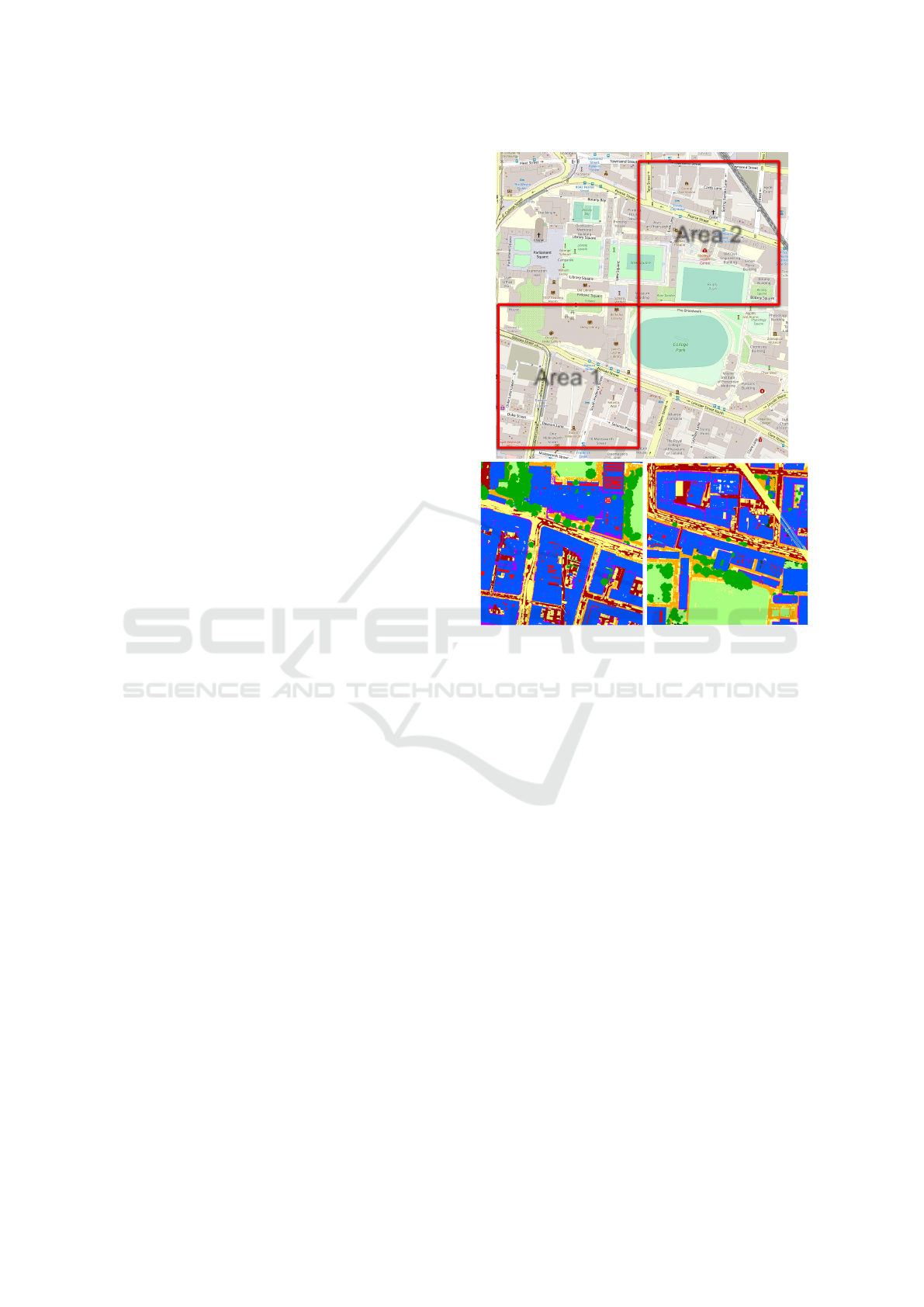
Figure 1: Areas evaluated in the benchmark. At the top,

the areas of the the city under study are overlaid in the map.

At the bottom, a top view of the ground truth of each area

is depicted with a different color per class. Area 1 is on the

left and Area 2 is on the right.

environments are the Kitti benchmark (Menze and

Geiger, 2015) and the TerraMobilita/iQmulus bench-

mark (Vallet et al., 2015). Both of them use 3D Mo-

bile Laser Scanning (MLS) as ground truth. The for-

mer includes the images captured alongside to evalu-

ate several tasks such as scene ﬂow, stereo, object de-

tection but it does not include neither aerial data nor

a speciﬁc MVS evaluation. The latter only provides

annotated 3D data, similar to the Paris-rue-madame

dataset (Serna et al., 2014) and the Oakland 3D Point

Cloud dataset (Munoz et al., 2009), but no images are

included and therefore the evaluation is done for tasks

like object segmentation and object classiﬁcation.

The Toronto/Vaihingen ISPRS benchmark used

in (Zhang et al., 2018) is not limited by the use of

MLS to create the ground-truth model. However, al-

though a large-scale urban scenario is covered, the 3D

building models are not created from the images, they

are created from the Aerial Laser Scan (ALS) point

cloud. Also, Urban Semantic 3D data (Bosch et al.,

2019) is a large-scale public dataset that includes se-

mantic labels for two large cities but it uses satellite

A Benchmark for 3D Reconstruction from Aerial Imagery in an Urban Environment

733

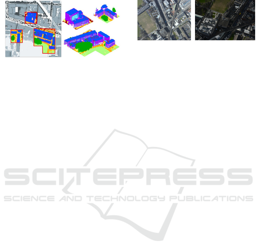
Figure 2: Hidden areas. On the left, an example of a hidden

area (in color) over the whole region (in grey). On the right,

the hidden area represented in 3D.

imagery and they do not provide a semantic evalua-

tion of the 3D reconstruction. The ISPRS Test project

on Urban Classiﬁcation and 3D Building Reconstruc-

tion (Rottensteiner et al., 2014) have airborne images

but the number of images offered is no more than 20

per area, the benchmark reconstruction task is focused

on roofs, the density of the ALS is 6 points per m

and they only provide one type of images per set. One

of the most recent annotated LiDAR point clouds cap-

tured with ALS is DublinCity (Zolanvari et al., 2019),

which also includes airborne images associated (Lae-

fer et al., 2015). The average density of the ALS

point cloud is remarkable compared to other existing

datasets (i.e., 348.43 points/m

) and the LiDAR point

cloud is used as ground truth for the evaluation of an

image-based 3D reconstruction, but they do not in-

clude the annotations in the evaluation.

3 BENCHMARK DATASET

Area Selection. The initial dataset of Dublin city cen-

ter (Laefer et al., 2015) and the annotations incorpo-

rated in (Zolanvari et al., 2019) are used for the cre-

ation of this benchmark. We analysed the whole an-

notated dataset (the potential ground truth) to ensure

that the selected areas constitute a good representation

of the city and also, that they have a balanced distri-

bution of points in each category, so content diversity

and representativeness is guaranteed for an evaluation

per urban object category. The criteria used to choose

the speciﬁc tiles for evaluation are based on the area

of the city covered, the variety of the city elements in

them and the avoidance of potential sources of errors.

In particular, we have discarded the ones that are

covering less than 250 × 250 m

of the city, the ones

that include less than 1% of points corresponding to

grass and less than 4% of points corresponding to

trees. Also, we discarded tiles with points in the unde-

ﬁned class above 10% and the ones containing cranes,

because they may degrade performance. With these

(a) (b)

Figure 3: Images. (a) a sample of the nadir set of images;

(b) a sample of the oblique one.

criteria two tiles are left, that will be the areas used in

this benchmark, shown in Fig. 1 and will allow us to

have a representative part of the city while keeping the

amount of data that have to be processed reasonable.

Hidden Areas. We are also evaluating a speciﬁc re-

gion in each area that will not be revealed to the user

to avoid ﬁne tuning during online evaluation (see Sec-

tion 4). We call these regions hidden areas and we

show an example of a potential hidden area in Fig. 2.

As it can be seen, they consist of meaningful sec-

tions of the city spread across the ground truth (each

of them including several classes). We have selected

them taking the class distribution into account but the

exact portions of the ground truth that belongs to the

hidden area are not revealed.

Area Description. We are evaluating two different

regions of the city of Dublin (depicted in red in Fig. 1)

which were selected following the aforementioned

analysis. Area 1 encompasses the south west part of

Trinity College Dublin (TCD) campus, several streets

of the city, buildings and green areas. Area 2 includes

the north east of the TCD campus, different buildings,

streets and it includes parts of rail tracks.

Table 1 shows the distribution of the classes in

terms of number of points and the percentage of

points in the whole ground truth and the hidden areas.

It can be seen that the most populated class is roof

and the one with least representation is doors. Never-

theless, the percentage of the class roof in the hidden

areas is more balanced with the other classes. It can

also be observed that the undeﬁned data, which is a

potential source of inaccuracies, represents between

5% and 9% of the points. Area 1 has almost double of

points in the window category and almost four times

of windows in the roof. Furthermore, Area 2 triples

the number of points associated with grass in Area 1.

For each area, three different sets of images are

used to create the reconstructions: oblique, nadir and

combined. Oblique and nadir contain images from

the homonyms groups explained in (Zolanvari et al.,

2019) and a sample of each group is shown in Fig. 3.

The combined group contains the images from both of

them. The initial dataset contains a large number of

oblique and nadir images, many more than needed for

VISAPP 2021 - 16th International Conference on Computer Vision Theory and Applications

734

Table 1: Number of points and percentage of points per class in each evaluated area. Also the number of points and percentage

used as the hidden zone.

undeﬁned

facade

window

door

roof

r. window

r. door

sidewalk

street

grass

tree

Area 1

# points (×10

) 1397 3048 540 40 10727 481 3 2029 3210 1587 3471

percentage 5.27 11.49 2.04 0.15 40.43 1.81 0.01 7.65 12.10 5.98 13.08

hidden # p. (×10

) 1015 1816 312 27 2849 247 2 1602 2441 1353 2720

hidden pct. 7.06 12.63 2.17 0.19 19.81 1.72 0.01 11.14 16.97 9.41 18.91

Area 2

# points (×10

) 1615 2776 308 40 7807 112 3 2789 2642 4061 2852

percentage 6.46 11.10 1.23 0.16 31.22 0.45 0.01 11.15 10.57 16.24 11.41

hidden # p. (×10

) 1262 1547 220 27 2708 47 1 2010 1993 2226 1897

hidden pct. 9.05 11.105 1.58 0.19 19.43 0.34 0.01 14.42 14.30 15.97 13.61

a meaningful 3D reconstruction of a particular area.

Further, it is not obvious which images are associated

with a certain area. In order to identify a meaning-

ful subset of images, we ran the COLMAP SfM al-

gorithm (Sch

onberger and Frahm, 2016) with all the

oblique images of the initial dataset. We then selected

the subset of images, where each generated at least

1500 3D points in the areas under evaluation. The

same process was done with the nadir images.

4 EVALUATION

Pipelines Tested. In this benchmark, we evaluate the

3D dense point cloud obtained when an image-based

reconstruction pipeline is applied to a collection of

aerial images. Usually, research is focused on solving

one speciﬁc problem of the pipeline: SfM or MVS.

However, we want to allow the possibility of evaluat-

ing new techniques that can solve the problem with

a different approach, not necessarily applying SfM

followed by MVS. Furthermore, as we are not in a

controlled environment, we do not have the camera

positions with accuracy to be used as ground-truth.

Instead, we have the GPS, which is only a coarse ap-

proximation. For these reasons, we are only evaluat-

ing the ﬁnal 3D reconstruction, not the intermediate

steps.

To do the state-of-the-art evaluation we have se-

lected different pipelines that were studied in the

latest comparison of open-source 3D reconstruction

methods (Stathopoulou et al., 2019). Following this

approach we established the pipelines assembling

compatible SfM and MVS methods. In particular,

for SfM, we use COLMAP (Sch

onberger and Frahm,

2016) which includes a geometric veriﬁcation strat-

egy to improve robustness on initialization and tri-

angulation and an improved bundle adjustment strat-

egy with an outlier ﬁltering strategy. Besides, we

selected OpenMVG with two different approaches:

global (Moulon et al., 2013), with a global calibra-

tion approach based on the fusion of relative mo-

tions between image pairs; and incremental (Moulon

et al., 2012), that iteratively adds new estimations to

an initial reconstruction minimizing the drift with suc-

cessive steps of non-linear reﬁnement. Furthermore,

for MVS, we choose COLMAP (Sch

onberger et al.,

2016) that makes a joint estimation of depth and nor-

mal information and makes a pixelwise view selec-

tion using photometric and geometric priors. We also

use OpenMVS (Sch

onberger et al., 2016), that uses

an efﬁcient patch based stereo matching followed by

a depth-map reﬁnement process. In (Stathopoulou

et al., 2019), AliceVision was also tested, but we

are not including it in our evaluation because it di-

rectly produces a mesh, without providing a dense

point cloud representation as an exploitable interme-

diate step. However, AliceVision is based on the

incremental OpenMVG (Moulon et al., 2012) and

the CMPMVS (Jancosek and Pajdla, 2011) which

can handle weakly textured surfaces. We selected

the former method for SfM but the latter is no

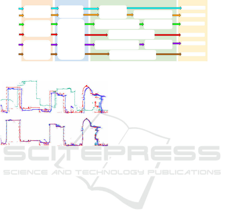
longer publicly available. To sum up, Fig. 4 shows

the details of the six pipelines tested in the bench-

mark: (1) COLMAP(SfM) + COLMAP(MVS); (2)

COLMAP(SfM) + OpenMVS; (3) OpenMVG-g +

COLMAP(MVS); (4) OpenMVG-g + OpenMVS; (5)

OpenMVG-i + COLMAP(MVS); (6) OpenMVG-i +

OpenMVS. The version of COLMAP, OpenMVG and

OpenMVS used are v3.6, v1.5 and v1.1 respectively,

and, as it is depicted in the ﬁgure, four stages are

needed: SfM, geo-registration, data preparation and

MVS. The SfM step includes the feature detection

and matching provided by each of the methods used.

The parameters used for COLMAP are the same as

in DublinCity (Zolanvari et al., 2019), and the param-

eters used for OpenMVG are the default: SIFT for

feature detection, essential matrix ﬁltering for com-

puting matches for global, and fundamental matrix

A Benchmark for 3D Reconstruction from Aerial Imagery in an Urban Environment

735

SfM Geo-registration MVS

Data preparation

OpenMVG

incremental

COLMAP

aligner

InterfaceCOLMAP

(OpenMVS)

OpenMVG2OpenMVS

(OpenMVG)

OpenMVG2COLMAP

(OpenMVG)

COLMAP

OpenMVG

global

OpenMVG

geodesy

registration

OpenMVG2OpenMVS

(OpenMVG)

OpenMVG2COLMAP

(OpenMVG)

Undistortion

(COLMAP)

Undistortion

(COLMAP)

Undistortion

(COLMAP)

COLMAP

OpenMVS

COLMAP

OpenMVS

COLMAP

OpenMVS

(1)

(2)

(3)

(4)

(5)

(6)

Figure 4: Scheme of 3D reconstruction pipelines tested. (1) COLMAP+COLMAP, (2) COLMAP+OpenMVS, (3) Open-

MVGg+COLMAP, (4) OpenMVGg+OpenMVS, (5) OpenMVGi+COLMAP, (6) OpenMVGi+OpenMVS.

Figure 5: Registration. Skyline of the ground-truth (in red)

against the 3D reconstructions with oblique (in green), nadir

(in purple) and the combined (in blue) sets of images. On

the top, the coarse registration, at the bottom, the ﬁne one.

ﬁltering for incremental. After the SfM is done, the

geo-information of the dataset is used for a coarse

registration of the point cloud (i.e, geo-registration),

and we use the methods provided by COLMAP and

OpenMVG.

After the geo-registration is done, we have to pre-

pare the data to be densiﬁed. For that reason, we use

the different procedures proposed for each method for

converting the formats and undistorting the images.

We used the same parameters each time we applied

the same procedure. Finally, the last step is the den-

siﬁcation which is done with the recommended pa-

rameters in COLMAP and OpenMVS except when

an image reduction was needed for OpenMVS. In that

case, we used the parameters reported in the ETH3D

benchmark which were not hard-coded.

Alignment. The strategies for the alignment of the

3D reconstructions with the ground truth usually con-

sist of two steps: a coarse alignment followed by the

reﬁnement of the initial estimation. In our evaluation,

the coarse registration is done in the geo-registration

step of the pipelines, and as a consequence, the dense

point clouds generated are already coarsely regis-

tered with the LiDAR scan. As an example, the re-

sults of the coarse registration with the COLMAP +

COLMAP pipeline are shown on the left in Fig. 5.

The skyline of the ground truth is depicted in red

and the 3D reconstructions in blue (oblique images),

green (nadir images) and purple (combined).

The reﬁnement of the registration is commonly

done applying a 7DoF ICP algorithm. This is the

strategy followed in (Knapitsch et al., 2017). A

more sophisticated approach is used in (Schops et al.,

2017), but they use the color information of the laser

scan, which is not available in our benchmark. In our

approach, we use the point cloud obtained from the

ﬁrst pipeline to reﬁne the coarse registration with the

ground-truth applying an ICP algorithm. Then, for

the rest of the pipelines, we use the camera positions

of the already reﬁned one as a reference, and we ap-

ply the same ICP algorithm to obtain the transforma-

tions that will align the cameras. After that, we ap-

ply the transformation to the entire 3D point clouds.

For online evaluation using our benchmark we will

require the input 3D point cloud to be already regis-

tered, which will allow users to use and optimize their

own registration.

Measurements. For the evaluation we use the mea-

surements proposed in (Knapitsch et al., 2017; Zolan-

vari et al., 2019). In particular, we use: precision, P,

recall, R and F score, F. The precision, shows how

closely the reconstruction is to the ground truth, the

recall, is related to how complete the reconstruction

is, and the F score, is a combination of both. Other

measurements as the mean distance between the point

clouds could be used as in (Stathopoulou et al., 2019),

but the advantage of the selected ones is that they are

less affected by outliers. They are deﬁned in Eq. (1),

Eq. (2), Eq. (3), respectively, for a given threshold dis-

tance d. In the equations, I is the point cloud under

evaluation and G is the ground-truth point cloud. |·| is

the cardinality and dist

I→G

(d) are the points in I with

a distance to G less than d and dist

G→I

(d) is analo-

gous (i.e., dist

A→B

(d) = {a ∈ A | min

b∈B

ka − bk

< d},

VISAPP 2021 - 16th International Conference on Computer Vision Theory and Applications

736

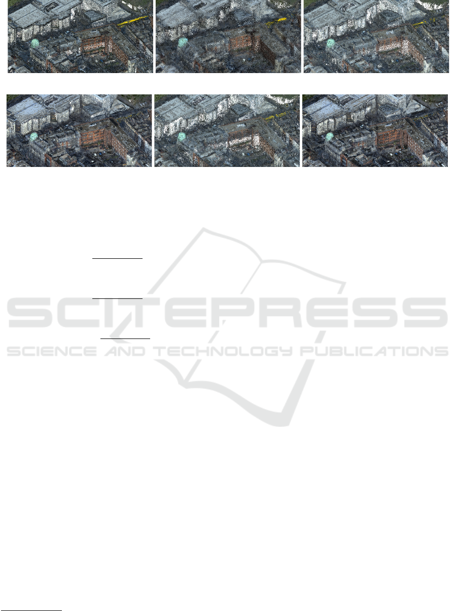
(a) (b) (c)

(d) (e) (f)

Figure 6: Qualitative 3D reconstruction results. Point clouds obtained with the oblique and nadir images combined in Area

1 with each of the pipelines tested (a) COLMAP + COLMAP, (b) COLMAP + OpenMVS, (c) OpenMVG-g + COLMAP, (d)

OpenMVG-g + OpenMVS, (e) OpenMVG-i + COLMAP, (f) OpenMVG-i + OpenMVS.

A and B being point clouds).

P(d) =

|dist

I→G

(d)|

|I|

100 (1)

R(d) =

|dist

G→I

(d)|

|G|

100 (2)

F(d) =

2P(d)R(d)

P(d) + R(d)

(3)

To perform the evaluation per class, the point under

evaluation will be given the same class as its nearest

neighbor in the ground-truth.

Online Evaluation. We will provide online eval-

uation

of the 3D reconstructions to stimulate and

support progress in the ﬁeld. The users should pro-

vide the ﬁnal dense point cloud already registered to

the ground truth. This will be possible because the

ground truth will be publicly available. To ensure a

fair comparison, we will be calculating the precision,

recall and F score not only in the complete ground

truth but also in the hidden areas.

5 RESULTS

We report the precision, recall and F score values for

each selected pipeline, set of images and area, includ-

ing the hidden parts. The measurements were calcu-

lated with d in the range of 1 cm to 100 cm obtain-

ing, as expected, an increasing performance in every

https://v-sense.scss.tcd.ie/research/6dof/benchmark-

3D-reconstruction

method when a further distance was considered. We

report the results at 25 cm, similar to (Zolanvari et al.,

2019), as a good compromise between the limitations

of the image resolution and the meaningfulness of the

precision, since selecting a very small distance would

mean poorer performances for all the methods and

with a larger distance the precision would be less in-

formative.

Scene Level Evaluation. Table 2 shows the evalu-

ation of the pipelines’ outcomes against the ground-

truth models without considering the urban element

category. From these measurements, we can ob-

serve that reconstructions from oblique imagery as in-

put, achieve the lowest recall values in all the areas.

Therefore, the precision has a main role in achieving

a high F score for this image set category. In particu-

lar, COLMAP + COLMAP has the best performance

(F score) with that type of imagery in every area. Ad-

ditionally, the reconstructions done with the nadir im-

age set have higher recall values than the ones with

the oblique imagery. Also, the recall is usually higher

than the precision for these sets so the accuracy is not

as determinant as in the oblique sets. As can be ob-

served, COLMAP + COLMAP is the best pipeline in

Area 1 whereas OpenMVG-i + OpenMVS is the best

in Area 2 (even in the hidden parts). These results

suggest that having different camera angles and less

coverage of the same parts of the scene (as it is the

case in the oblique set and not in the nadir one) makes

the recall value decrease while the precision remains

similar.

For the reconstructions obtained with the com-

bined imagery, OpenMVG-g + OpenMVS and

OpenMVG-i + OpenMVS have the highest F score:

A Benchmark for 3D Reconstruction from Aerial Imagery in an Urban Environment

737

Table 2: Quantitative results with the whole ground-truth. Each row shows the results of a speciﬁc 3D reconstruction

pipeline giving the precision / recall / F score for d=25cm obtained for the reconstruction in each set of images in each area.

The best score for each area and image set is in bold letters and the pipelines are as follow: (1) COLMAP + COLMAP,

(2) COLMAP + OpenMVS, (3) OpenMVG-g + COLMAP, (4) OpenMVG-g + OpenMVS, (5) OpenMVG-i + COLMAP, (6)

OpenMVG-i + OpenMVS.

Area 1 Area 2

oblique nadir oblique and nadir oblique nadir oblique and nadir

(1) 79.18 / 60.5 / 68.59 73.08 / 68.98 / 70.97 74.89 / 74.15 / 74.52 80.48 / 65.51 / 72.23 74.97 / 72.34 / 73.63 76.54 / 77.98 / 77.25

(2) 22.74 / 28.28 / 25.21 23.96 / 46.23 / 31.57 27.93 / 60.84 / 38.29 26.85 / 41.81 / 32.7 24.45 / 49.96 / 32.83 24.7 / 63.53 / 35.57

(3) 49.42 / 13.09 / 20.69 44.02 / 47.95 / 45.9 48.74 / 58.24 / 53.07 36.92 / 15.7 / 22.03 33.26 / 36.4 / 34.76 41.94 / 50.3 / 45.74

(4) 61.07 / 57.1 / 59.02 56.61 / 73.46 / 63.94 78.27 / 80.49 / 79.36 40.23 / 54.27 / 46.21 75.2 / 75.92 / 75.56 79.3 / 82.03 / 80.64

(5) 37.13 / 16.59 / 22.94 36.59 / 43.62 / 39.8 39.48 / 51.36 / 44.64 38.11 / 15.11 / 21.64 43.76 / 52.0 / 47.52 36.62 / 48.53 / 41.74

(6) 55.12 / 64.37 / 59.39 49.14 / 70.75 / 58.0 74.19 / 79.5 / 76.76 58.52 / 70.43 / 63.92 71.44 / 79.0 / 75.03 79.77 / 82.54 / 81.13

hidden Area 1 hidden Area 2

oblique nadir oblique and nadir oblique nadir oblique and nadir

(1) 78.68 / 49.89 / 61.06 72.69 / 62.77 / 67.37 74.54 / 68.34 / 71.3 80.06 / 61.48 / 69.55 73.63 / 68.9 / 71.18 75.5 / 75.27 / 75.39

(2) 23.55 / 18.97 / 21.01 24.42 / 36.88 / 29.39 28.38 / 50.45 / 36.32 27.05 / 37.02 / 31.26 24.24 / 43.98 / 31.25 24.4 / 56.88 / 34.15

(3) 43.12 / 6.61 / 11.46 42.52 / 38.01 / 40.14 48.48 / 48.74 / 48.61 36.47 / 13.19 / 19.37 33.08 / 31.82 / 32.43 40.97 / 43.7 / 42.29

(4) 56.57 / 48.7 / 52.34 56.03 / 69.48 / 62.03 75.36 / 75.76 / 75.56 40.31 / 54.08 / 46.19 74.93 / 74.31 / 74.62 77.19 / 79.52 / 78.34

(5) 30.83 / 8.88 / 13.79 36.51 / 35.47 / 35.98 38.79 / 42.08 / 40.37 35.24 / 12.3 / 18.24 43.7 / 47.28 / 45.42 35.35 / 42.39 / 38.55

(6) 52.93 / 59.33 / 55.95 48.47 / 67.81 / 56.53 70.56 / 75.02 / 72.72 56.16 / 67.58 / 61.34 67.99 / 77.08 / 72.25 78.38 / 80.49 / 79.42

Table 3: Quantitative results per urban element. Results for F score (top), precision (middle) and recall (bottom) for Area

1 and Area 2 at d=25cm. Each row gives the result for a particular class, ﬁrst in the whole area and then in the hidden area,

separated with a hyphen. The best score obtained among the pipelines is shown with the pipeline that generated it in brackets,

numbered as in Fig. 4. In bold, the best measurement per class among all the image sets in both areas. Pipelines are as follow:

(1) COLMAP + COLMAP, (2) COLMAP + OpenMVS, (3) OpenMVG-g + COLMAP, (4) OpenMVG-g + OpenMVS, (5)

OpenMVG-i + COLMAP, (6) OpenMVG-i + OpenMVS.

F SCORE

Area 1 - Area 1 hidden Area 2 - Area 2 hidden

oblique nadir combined oblique nadir combined

facade 58.34 (1) - 57.1 (1) 59.96 (4) - 59.08 (4) 67.01 (4) - 65.91 (4) 63.12 (1) - 62.17 (1) 67.7 (6) - 65.82 (6) 71.73 (6) - 70.83 (6)

window 58.83 (1) - 58.18 (1) 53.92 (4) - 53.83 (4) 62.41 (1) - 62.45 (1) 55.06 (1) - 57.2 (1) 61.73 (6) - 60.9 (6) 63.34 (6) - 63.59 (6)

door 41.97 (1) - 45.46 (1) 51.55 (4) - 52.55 (4) 53.14 (4) - 52.96 (4) 49.18 (6) - 48.63 (6) 53.84 (6) - 51.07 (6) 56.57 (6) - 56.69 (6)

roof 80.78 (1) - 75.55 (1) 80.18 (1) - 77.39 (1) 87.98 (4) - 85.55 (4) 81.57 (1) - 80.66 (1) 81.41 (1) - 80.06 (1) 86.05 (6) - 85.53 (6)

r. window 77.33 (1) - 77.67 (1) 73.78 (1) - 74.68 (1) 85.06 (4) - 85.04 (4) 74.54 (1) - 74.53 (1) 76.36 (6) - 78.54 (6) 83.0 (4) - 84.89 (6)

r. door 57.72 (1) - 65.94 (4) 53.58 (4) - 58.63 (3) 63.83 (4) - 69.3 (4) 50.1 (6) - 45.14 (1) 53.29 (6) - 41.27 (4) 50.71 (6) - 43.13 (6)

sidewalk 76.46 (6) - 74.99 (6) 79.76 (1) - 79.85 (1) 87.86 (4) - 87.42 (4) 79.11 (1) - 80.05 (1) 87.56 (4) - 87.14 (4) 88.28 (6) - 88.03 (6)

street 77.28 (1) - 74.91 (1) 85.85 (1) - 85.9 (1) 90.72 (4) - 90.78 (4) 71.02 (1) - 68.67 (1) 90.88 (4) - 90.55 (4) 90.81 (6) - 90.5 (6)

grass 84.12 (6) - 82.76 (6) 79.75 (1) - 77.38 (1) 88.79 (4) - 87.97 (4) 91.1 (1) - 89.1 (1) 95.59 (4) - 93.6 (4) 96.36 (6) - 94.91 (6)

tree 31.74 (6) - 32.55 (6) 38.47 (4) - 38.37 (4) 40.92 (1) - 40.21 (6) 25.34 (1) - 28.09 (1) 33.7 (1) - 35.08 (1) 39.45 (1) - 41.34 (1)

PRECISION

Area 1 - Area 1 hidden Area 2 - Area 2 hidden

oblique nadir combined oblique nadir combined

facade 75.23 (1) - 75.84 (1) 61.32 (1) - 62.59 (1) 66.9 (1) - 68.04 (1) 73.77 (1) - 74.81 (1) 66.71 (6) - 64.7 (6) 68.33 (1) - 69.01 (1)

window 64.97 (1) - 65.13 (1) 54.16 (1) - 56.04 (1) 60.75 (1) - 62.14 (1) 63.77 (1) - 63.84 (1) 56.53 (6) - 55.17 (6) 59.09 (1) - 59.16 (1)

door 59.1 (1) - 58.75 (1) 42.31 (4) - 43.6 (4) 47.34 (1) - 46.05 (1) 55.49 (1) - 54.64 (1) 49.25 (6) - 45.61 (6) 48.06 (4) - 48.44 (6)

roof 81.56 (1) - 80.58 (1) 77.05 (1) - 74.96 (1) 84.08 (4) - 80.21 (4) 83.21 (1) - 83.35 (1) 78.56 (1) - 77.46 (1) 81.16 (6) - 80.91 (6)

r. window 78.96 (1) - 80.13 (1) 70.18 (1) - 72.01 (1) 79.43 (4) - 78.29 (4) 81.25 (1) - 83.9 (1) 80.25 (1) - 82.71 (1) 80.65 (1) - 84.08 (1)

r. door 63.5 (1) - 62.5 (1) 48.32 (1) - 55.11 (4) 54.66 (1) - 59.58 (1) 65.19 (1) - 63.67 (1) 45.04 (6) - 40.6 (4) 45.99 (6) - 40.99 (1)

sidewalk 88.51 (1) - 88.48 (1) 80.37 (1) - 81.26 (1) 83.35 (4) - 83.16 (1) 87.79 (1) - 87.55 (1) 83.66 (4) - 83.26 (4) 82.67 (6) - 82.32 (6)

street 90.97 (1) - 90.86 (1) 83.27 (1) - 83.28 (1) 86.43 (4) - 86.35 (4) 87.23 (1) - 86.92 (1) 86.71 (4) - 86.46 (4) 85.91 (6) - 85.87 (6)

grass 92.32 (1) - 91.33 (1) 84.18 (1) - 82.37 (1) 89.35 (4) - 88.73 (4) 95.91 (1) - 94.75 (1) 96.11 (4) - 94.39 (4) 95.88 (4) - 94.15 (6)

tree 78.37 (1) - 77.2 (1) 75.41 (4) - 75.15 (4) 74.22 (1) - 72.94 (1) 80.73 (1) - 80.49 (1) 77.41 (6) - 76.66 (6) 77.63 (1) - 77.23 (1)

RECALL

Area 1 - Area 1 hidden Area 2 - Area 2 hidden

oblique nadir combined oblique nadir combined

facade 47.64 (1) - 45.78 (1) 63.92 (4) - 62.69 (4) 72.38 (4) - 71.14 (4) 60.48 (6) - 56.97 (6) 68.72 (6) - 66.99 (6) 77.28 (6) - 75.63 (6)

window 53.75 (1) - 52.58 (1) 62.35 (4) - 61.28 (4) 78.64 (4) - 77.22 (4) 56.4 (6) - 54.72 (6) 67.99 (6) - 67.96 (6) 77.05 (6) - 77.71 (6)

door 40.86 (6) - 40.72 (6) 65.95 (4) - 66.12 (4) 68.76 (4) - 67.99 (4) 51.1 (6) - 54.05 (6) 59.37 (6) - 58.03 (6) 68.94 (6) - 68.34 (6)

roof 80.03 (1) - 76.27 (6) 83.82 (4) - 83.92 (4) 92.25 (4) - 91.65 (4) 80.08 (6) - 81.01 (6) 87.8 (6) - 88.35 (6) 91.57 (6) - 90.72 (6)

r. window 75.76 (1) - 84.01 (6) 77.75 (1) - 77.57 (1) 91.54 (4) - 93.07 (4) 70.23 (6) - 72.07 (6) 79.95 (6) - 84.97 (6) 85.78 (4) - 87.82 (6)

r. door 56.41 (4) - 71.34 (4) 63.3 (3) - 70.56 (3) 83.51 (4) - 92.79 (4) 60.73 (6) - 35.79 (6) 65.25 (6) - 42.42 (6) 65.8 (4) - 56.62 (6)

sidewalk 79.36 (6) - 77.95 (6) 90.37 (4) - 91.4 (4) 92.88 (4) - 92.56 (4) 84.66 (6) - 84.74 (6) 93.77 (6) - 93.31 (6) 94.71 (6) - 94.59 (6)

street 80.46 (6) - 79.17 (6) 92.97 (4) - 92.75 (4) 95.45 (4) - 95.68 (4) 77.66 (6) - 73.99 (6) 95.47 (4) - 95.05 (4) 96.31 (6) - 95.66 (6)

grass 81.14 (6) - 79.23 (6) 75.77 (1) - 74.63 (4) 88.45 (6) - 87.43 (6) 86.75 (1) - 84.09 (1) 95.08 (4) - 92.82 (4) 96.88 (6) - 95.67 (6)

tree 20.94 (6) - 21.65 (6) 25.82 (4) - 25.8 (6) 29.44 (2) - 28.76 (2) 15.03 (1) - 17.01 (1) 21.62 (1) - 22.82 (1) 26.58 (2) - 30.28 (2)

VISAPP 2021 - 16th International Conference on Computer Vision Theory and Applications

738

the former in Area 1 and latter in Area 2. Fig. 6 also

includes the qualitative results of the point clouds ob-

tained for the combined dataset in Area 1 rendered un-

der the same conﬁguration (e.g., point size, shading)

to make them comparable. From these results, we can

observe that the point cloud obtained with COLMAP

+ COLMAP (Fig. 6 (a)) is sharper than the one ob-

tained with COLMAP + OpenMVS (Fig. 6 (b)), in ac-

cordance with the precision values (74.89 and 27.93,

respectively). Moreover, there are also differences in

the completeness of the reconstructions: OpenMVG-i

+ OpenMVS (Fig. 6 (f)) and OpenMVG-g + Open-

MVS (Fig. 6 (d)) are denser than the rest, and they

also seem to be accurate. As before, the F score val-

ues conﬁrm these observations, where they obtained

the highest scores (79.36 and 76.76).

Urban Category Centric Evaluation. Additionally,

in Table 3 we present a summary of the same mea-

surements calculated above (precision, recall and F

score) but this time per urban element category. This

summary shows three tables, one per measurement,

where each row has the results of a speciﬁc class (i.e.,

urban category) and each column corresponds to a

unique set of images. The result presented per cell in

the table is the maximum score obtained among the

six pipelines tested (see Fig. 4) and the pipeline that

generate it is shown in brackets. The results for the

complete area and the hidden one are presented in the

same cell, in that order, separated by a hyphen.

Analyzing the results that were obtained per class

across all the image sets available, we can observe

that the method that most frequently gets the maxi-

mum precision is COLMAP + COLMAP. Those re-

sults are different when looking at recall. In that case,

the pipeline OpenMVG-i + OpenMVS is the one that

more frequently achieves the highest scores. When

looking at the F score, we cannot identify a clear

predominant pipeline for each class. In all the sce-

narios, the class with lowest F score values is tree

and the results are really inﬂuenced by the low val-

ues of the recall. These results conﬁrm the hypoth-

esis in (Zolanvari et al., 2019): trees in the parks of

the city can degrade the scores of the reconstructions.

We can also analyze the results related to the image

set under study. For example, with the combined set,

the pipeline with best performance in the majority of

classes is OpenMVG-g + OpenMVS in Area 1 and

OpenMVG-i + OpenMVS in Area 2. These results

are in accordance with the ones commented before,

which does not consider the class information (Ta-

ble 2).

There is a different case scenario when we look at

the results with the nadir images. In Area 2 the scores

from the OpenMVG-i + OpenMVS pipeline are the

highest in most of the classes but it is not the best

pipeline in the scene level evaluation. This is because

OpenMVG-i + OpenMVS is the best with the facade

class, with 11.10% of occupancy in the ground-truth

(see Table 1), but also in classes with 1.23% of occu-

pancy or less. However, OpenMVG-g + OpenMVS

achieves the highest scores in the classes grass, side-

walk and street (16.24%, 11.18% and 10.57% of oc-

cupancy, respectively) and they also have the high-

est scores among all the classes. Also, if we look

at the scores per class with the combined set in Area

1, COLMAP + COLMAP and OpenMVG-g + Open-

MVS obtain the highest F scores in the same num-

ber of classes. This time, the most populated classes

are the ones where COLMAP + COLMAP is better.

These results reﬂect the importance of incorporating

an object-category centric evaluation since a more de-

tailed analysis can be done. The results of the evalua-

tion per urban category in the hidden part (also de-

picted in Table 3) are different from the ones with

the whole area but still follow the same pattern. For

example, we can observe that the method that gener-

ates the best results per image set and class remains

constant for the majority of them except for the door

class. This is due to its small amount of samples.

Evaluation of Pipeline Components. We can

also observe that, in general, the pipelines that ob-

tained the best results are COLMAP + COLMAP,

OpenMVG-g + OpenMVS and OpenMVG-i + Open-

MVS. These results are in accordance with previ-

ous studies that used the same kind of metric, where

COLMAP + COLMAP and OpenMVG-i + Open-

MVS obtained the best results (Knapitsch et al.,

2017). In particular, in that study OpenMVG-g +

OpenMVS never has better results than COLMAP

+ COLMAP, but this situation is plausible in our

study given the different camera trajectories (aerial

grid conﬁguration vs circle around an object), soft-

ware versions and parameters used. COLMAP used

as MVS is better than OpenMVS only if it is applied

after COLMAP SfM. Whereas OpenMVS is better

using the other SfM methods tested. This leads to the

necessity to test not only a particular MVS method

but a complete pipeline since it is going to be inﬂu-

enced by: the results obtained in the SfM step, the

data conversion and preparation for the MVS step, as

well as memory and computing limitations. In this

benchmark, the results after each step are not evalu-

ated because, as explained in Section 4, we want to

enforce the creation of end-to-end solutions and we

do not focus on any particular part of a pipeline. Sim-

ilarly, speciﬁc processing times are not reported but

for all the pipelines it was in the order of hours due to

the quantity of images that had to be processed.

A Benchmark for 3D Reconstruction from Aerial Imagery in an Urban Environment

739

6 CONCLUSION

In this paper, we have presented a novel bench-

mark for evaluating image-based 3D reconstruction

pipelines with aerial images in urban environments.

The results obtained with the considered SfM+MVS

state-of-the-art pipelines are evaluated at scene level

and per urban category. This allows for further

analysis of the reconstructions (i.e., analysis of

the inﬂuence of each urban category in the scene

level scores) and it supports previous hypothesis

(e.g., parks can degrade the F score values in a

scene level evaluation) with quantitative measure-

ments. Also, we provide the means for evaluating

results in a hidden area to avoid ﬁne tuning of

algorithms to the given ground truth. Furthermore,

we stimulate and support the evaluation of new

approaches for image-based 3D reconstruction as

we do not limit the evaluation to a speciﬁc stage

of the pipeline (e.g., MVS). Finally, to support the

progress of research in the community we provide

the dataset and an online evaluation platform at

https://v-sense.scss.tcd.ie/research/6dof/benchmark-

3D-reconstruction.

ACKNOWLEDGEMENTS

This publication has emanated from research con-

ducted with the ﬁnancial support of Science Foun-

dation Ireland (SFI) under the Grant Number

15/RP/2776.

REFERENCES

Aanæs, H., Jensen, R. R., Vogiatzis, G., Tola, E., and Dahl,

A. B. (2016). Large-scale data for multiple-view stere-

opsis. International Journal of Computer Vision.

Barnes, C., Shechtman, E., Finkelstein, A., and Goldman,

D. B. (2009). Patchmatch: A randomized correspon-

dence algorithm for structural image editing. In ACM

Transactions on Graphics (ToG). ACM.

Bosch, M., Foster, K., Christie, G., Wang, S., Hager, G. D.,

and Brown, M. (2019). Semantic stereo for incidental

satellite images. In WACV 2019. IEEE.

Furukawa, Y. and Ponce, J. (2010). Accurate, dense, and ro-

bust multiview stereopsis. IEEE Transactions on Pat-

tern Analysis and Machine Intelligence.

Hartley, R. and Zisserman, A. (2003). Multiple view geom-

etry in computer vision. Cambridge University Press.

Jancosek, M. and Pajdla, T. (2011). Multi-view reconstruc-

tion preserving weakly-supported surfaces. In CVPR

2011. IEEE.

Knapitsch, A., Park, J., Zhou, Q.-Y., and Koltun, V. (2017).

Tanks and temples: Benchmarking large-scale scene

reconstruction. ACM Transactions on Graphics.

Laefer, D. F., Abuwarda, S., Vo, A.-V., Truong-Hong, L.,

and Gharibi, H. (2015). 2015 aerial laser and pho-

togrammetry survey of dublin city collection record.

Menze, M. and Geiger, A. (2015). Object scene ﬂow for

autonomous vehicles. In CVPR 2015.

Moulon, P., Monasse, P., and Marlet, R. (2012). Adaptive

structure from motion with a contrario model estima-

tion. In ACCV 2012. Springer Berlin Heidelberg.

Moulon, P., Monasse, P., and Marlet, R. (2013). Global fu-

sion of relative motions for robust, accurate and scal-

able structure from motion. In ICCV 2013.

Munoz, D., Bagnell, J. A., Vandapel, N., and Hebert, M.

(2009). Contextual classiﬁcation with functional max-

margin markov networks. In CVPR 2009.

Ozdemir, E., Toschi, I., and Remondino, F. (2019). A multi-

purpose benchmark for photogrammetric urban 3d re-

construction in a controlled environment.

Pag

es, R., Amplianitis, K., Monaghan, D., Ond

rej, J., and

Smoli

c, A. (2018). Affordable content creation for

free-viewpoint video and vr/ar applications. Journal

of Visual Communication and Image Representation.

Rottensteiner, F., Sohn, G., Gerke, M., Wegner, J. D., Bre-

itkopf, U., and Jung, J. (2014). Results of the isprs

benchmark on urban object detection and 3d building

reconstruction. ISPRS journal of photogrammetry and

remote sensing.

Ruano, S., Cuevas, C., Gallego, G., and Garc

ıa, N. (2017).

Augmented reality tool for the situational awareness

improvement of uav operators. Sensors.

Ruano, S., Gallego, G., Cuevas, C., and Garc

ıa, N. (2014).

Aerial video georegistration using terrain models from

dense and coherent stereo matching. In Geospatial In-

foFusion and Video Analytics IV; and Motion Imagery

for ISR and Situational Awareness II. International So-

ciety for Optics and Photonics.

Sch

onberger, J. L. and Frahm, J.-M. (2016). Structure-

from-motion revisited. In CVPR 2016.

Sch

onberger, J. L., Zheng, E., Pollefeys, M., and Frahm, J.-

M. (2016). Pixelwise view selection for unstructured

multi-view stereo. In ECCV 2016. Springer.

Schops, T., Schonberger, J. L., Galliani, S., Sattler, T.,

Schindler, K., Pollefeys, M., and Geiger, A. (2017).

A multi-view stereo benchmark with high-resolution

images and multi-camera videos. In CVPR 2017.

Seitz, S. M., Curless, B., Diebel, J., Scharstein, D., and

Szeliski, R. (2006). A comparison and evaluation of

multi-view stereo reconstruction algorithms. In CVPR

2006.

Serna, A., Marcotegui, B., Goulette, F., and Deschaud, J.-

E. (2014). Paris-rue-madame database: a 3d mobile

laser scanner dataset for benchmarking urban detec-

tion, segmentation and classiﬁcation methods.

Snavely, N., Seitz, S. M., and Szeliski, R. (2008). Modeling

the world from internet photo collections. Interna-

tional Journal of Computer Vision.

Stathopoulou, E. K., Welponer, M., and Remondino, F.

(2019). Open-source image-based 3d reconstruction

VISAPP 2021 - 16th International Conference on Computer Vision Theory and Applications

740

pipelines: review, comparison and evaluation. The

International Archives of Photogrammetry, Remote

Sensing and Spatial Information Sciences.

Strecha, C., Von Hansen, W., Van Gool, L., Fua, P., and

Thoennessen, U. (2008). On benchmarking camera

calibration and multi-view stereo for high resolution

imagery. In CVPR 2008.

Sweeney, C., Hollerer, T., and Turk, M. (2015). Theia:

A fast and scalable structure-from-motion library. In

Proceedings of the ACM International Conference on

Multimedia, pages 693–696. ACM.

Vallet, B., Br

edif, M., Serna, A., Marcotegui, B., and Papar-

oditis, N. (2015). Terramobilita/iqmulus urban point

cloud analysis benchmark. Computers & Graphics.

Zhang, L., Li, Z., Li, A., and Liu, F. (2018). Large-scale

urban point cloud labeling and reconstruction. ISPRS

Journal of Photogrammetry and Remote Sensing.

Zolanvari, S., Ruano, S., Rana, A., Cummins, A., da Silva,

R. E., Rahbar, M., and Smolic, A. (2019). Dublincity:

Annotated lidar point cloud and its applications. 30th

BMVC.

A Benchmark for 3D Reconstruction from Aerial Imagery in an Urban Environment

741