3D Object Classiﬁcation via Part Graphs

Florian Teich

, Timo L

uddecke

and Florentin W

org

otter

III. Physikalisches Institut, Georg-August Universit

at G

ottingen, Friedrich-Hund-Platz 1, G

ottingen, Germany

Keywords:

3D Classiﬁcation, Segmentation, Graphs.

Abstract:

3D object classiﬁcation often requires extraction of a global shape descriptor in order to predict the object class.

In this work, we propose an alternative part-based approach. This involves automatically decomposing objects

into semantic parts, creating part graphs and employing graph kernels on these graphs to classify objects based

on the similarity of the part graphs. By employing this bottom-up approach, common substructures across

objects from training and testing sets should be easily identiﬁable and may be used to compute similarities

between objects. We compare our approach to state-of-the art methods relying on global shape description

and obtain superior performance through the use of part graphs.

1 INTRODUCTION

Classifying objects based on their shape and appear-

ance is essential to many applications such as au-

tonomous vehicles, assistive robots and scene un-

derstanding. For example in robotics, it is crucial

for 3D shape classiﬁcation algorithms to make cor-

rect predictions about what class an object belongs

to. Driven by the trend of 2.5D- and 3D-devices be-

coming cheaper, the focus on 3D vision tasks has in-

creased recently. State-of-the-art methods (Qi et al.,

2017b; Kanezaki et al., 2018) usually treat the ob-

ject as a whole, reduce the global shape to a global

3D feature - explicitly or implicitly encoded - and

employ classiﬁcation techniques such as Multi-Layer-

Perceptrons (Qi et al., 2017a), single Fully-Connected

layer (Li et al., 2018; Kanezaki et al., 2018) or Sup-

port Vector Machines (SVMs) (Yang et al., 2017; Su

et al., 2015; Yu et al., 2018; Wang et al., 2019a)

to learn distinguishing different object classes. This

global approach fails to make explicit use of seman-

tic substructures of the objects: their parts. Object

concepts like tables often consist of parts, i.e. a

tabletop and a few legs. Decomposing objects into

their parts and reasoning about the object classes us-

ing these parts might show much better generalization

than standard techniques that only use global 3D de-

scriptors. Substructures already seen in the training

set can be exploited to increase the certainty that the

https://orcid.org/0000-0001-6708-7233

https://orcid.org/0000-0002-1643-7827

https://orcid.org/0000-0001-8206-9738

object belongs to a speciﬁc class. For instance, dur-

ing training time only table instances with four table

legs may be seen, the test set may consist of tables

with many more legs. In this case, systems that make

use of part graphs are able to identify common struc-

tures in the tables from the training and the test set

and associate these instances from the same class eas-

ily, whereas classical methods may fail.

In his theory of Recognition-by-Components

(Biederman, 1987), Biederman theorizes that humans

perceive objects as compositions of volumetric primi-

tives - geons - and recognize objects based on them

in a bottom-up manner. Following this theory, we

present a pipeline to classify 3D shapes by ﬁrst de-

composing an object into its parts, creating attributed

part graphs and ﬁnally classifying these graphs to pre-

dict the shapes’ classes.

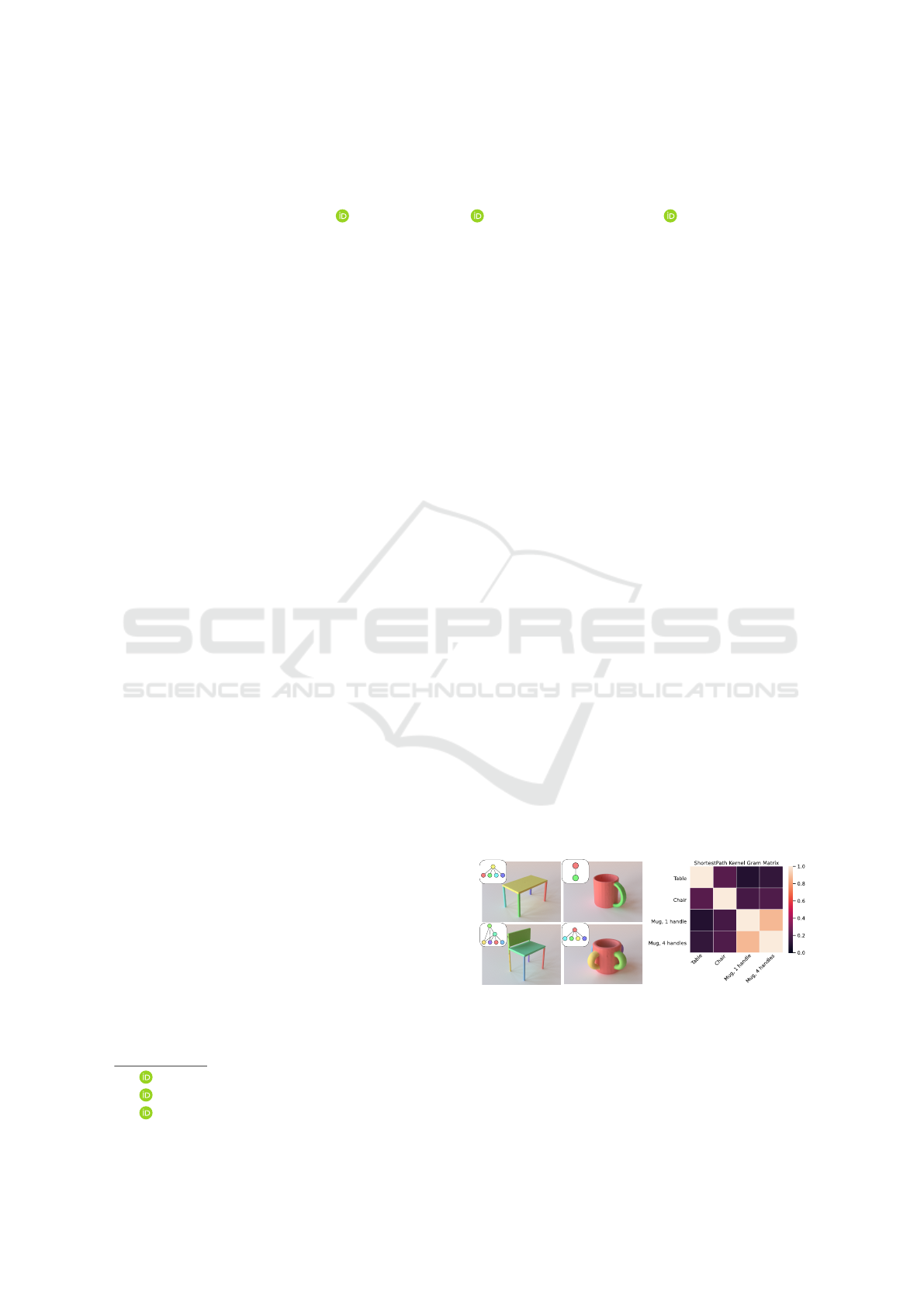
Figure 1: Objects are automatically segmented and part

graphs are created. Shape descriptors of parts serve as node

attributes in the graph. Relying on this, graph kernels can

be used to estimate similarity of objects.

Teich, F., Lüddecke, T. and Wörgötter, F.

3D Object Classiﬁcation via Part Graphs.

DOI: 10.5220/0010232604170426

In Proceedings of the 16th International Joint Conference on Computer Vision, Imaging and Computer Graphics Theory and Applications (VISIGRAPP 2021) - Volume 5: VISAPP, pages

417-426

ISBN: 978-989-758-488-6

417

VHV, ESF, FoldingNet

SP, GH, WWL

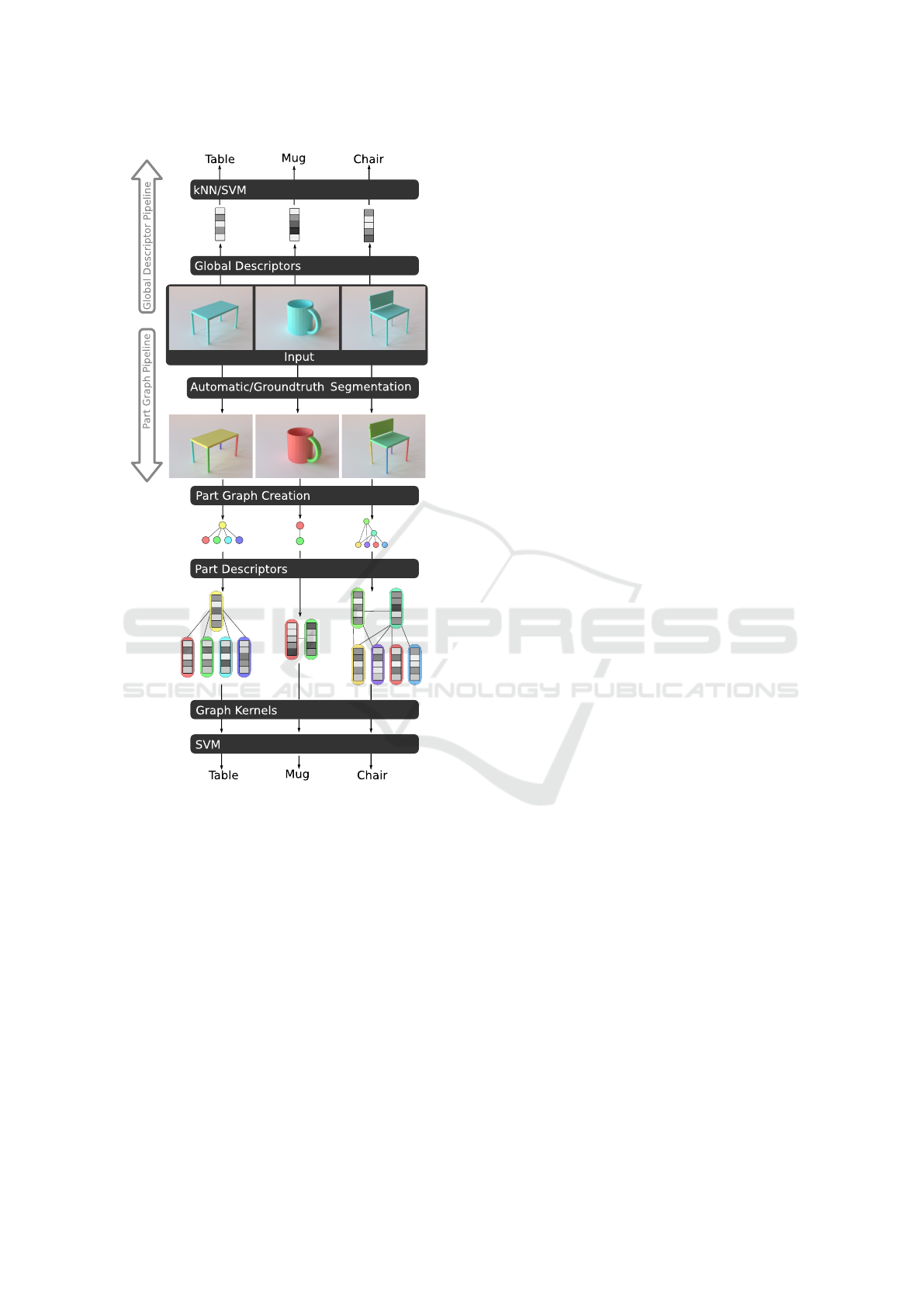
Figure 2: Overview for global descriptor pipeline and the

part graph pipeline. For the former, global descriptors are

extracted from the input shapes (here either VFH, ESF

or FoldingNet), which are fed to the SVM. For the part

graph pipeline, the input shape is ﬁrst decomposed into its

parts, using groundtruth- or automatic segmentation. Sub-

sequently, the part graph is created and the parts’ descriptors

are extracted (again, either VFH, ESF or FoldingNet de-

scriptors). Finally, graph kernels (ShortestPath, GraphHop-

per or Wasserstein Weisfeiler-Lehman) are used to compute

the kernel matrix between all graphs to train a SVM.

2 METHOD OVERVIEW

For the decomposition of objects into parts, various

segmentation algorithms already exist that try to ﬁnd

part boundaries on the surface to result in a part clus-

tering of the object. Afterwards, a graph is created

where nodes represent part instances of the object

and edges indicate spatial adjacency of these part in-

stances. This process is illustrated in Fig. 2. Differ-

ent objects may contain a different number of parts,

therefore it is not straightforward how to compute

similarities between the obtained part graphs. In this

work we employ graph kernels to solve this problem.

Furthermore, we compare ground truth segmentations

and automatic segmentations that result in different

part-graphs and employ various 3D shape descriptors

in order to benchmark our approach against classical

classiﬁcation methods as k-Nearest-Neighbor (kNN)

and Support Vector Machines on the global shape de-

scriptors.

The underlying hypothesis of this work is that an

explicit decomposition into parts helps in identifying

untypical objects. Our contributions are:

• A comparison of different graph kernels on part

graphs,

• the identiﬁcation of useful node attributes (3D de-

scriptors) for the part graphs,

• a benchmark against global shape descriptor clas-

siﬁers.

• and the estimation of the potential of this method

when an optimal segmentation is present.

3 RELATED WORKS

3.1 Classical 2D Image Classiﬁcation

Object classiﬁcation is one of the central problems

in Computer Vision. Given a set of possible classes

and a query object, the task is to decide which class

the object belongs to. Most traditional image classi-

ﬁers start by extracting features such as SIFT (Lowe,

1999) or SURF (Bay et al., 2006) from the image. In

different images, a varying amount of keypoints and

patches may be detected and reduced to their feature

vectors, making it non-trivial to compare two sets (of

different sizes) of feature vectors extracted from dif-

ferent images. The Bag-of-visual-words (Sivic and

Zisserman, 2003) method tackles this issue by iden-

tifying codewords (cluster centroids of the feature

vectors found in the training set). All feature vec-

tors detected inside an image are then classiﬁed as

codewords and the image can be reduced to the his-

togram of codewords present inside. A classiﬁer, e.g.

an SVM (Cortes and Vapnik, 1995) can then be em-

ployed to classify a query image based on its ﬁxed

size feature histogram.

VISAPP 2021 - 16th International Conference on Computer Vision Theory and Applications

418

3.2 3D Shape Classiﬁcation

Ideas and concepts from 2D classiﬁcation have been

widely adopted in 3D shape classiﬁcation.

In (Bronstein et al., 2011), a set of 3D feature

descriptors were used to create bag-of-visual-words

for shape classiﬁcation and retrieval, analogous to 2D

image classiﬁers (Sivic and Zisserman, 2003; Fei-Fei

and Perona, 2005).

Maturana et al. (Maturana and Scherer, 2015) use

a 3D CNN to classify voxelized representations of 3D

shapes. Their method suffers from discretization of

the input shapes and long training times due to the

additional dimension compared to 2D CNNs.

The Multi-view method in (Su et al., 2015) ren-

ders the 3D object from different views and applies a

CNN on these input images. The activations from the

different views are merged by using a max-pool op-

eration and sent to the second CNN. At testing time,

activations in the last layer of the ﬁrst CNN for all

different views are evaluated and each is fed to a one-

vs-rest linear SVMs. The predictions of the SVMs

are summed up and the highest scoring class is used

as the ﬁnal class prediction. This multi-view method

leads to highly accurate classiﬁers in many cases, of-

ten surpassing performance of pure 3D methods (Qi

et al., 2016).

Another popular 3D object classiﬁcation method

is the Deep Neural Network architecture PointNet (Qi

et al., 2017a). PointNet transforms the input point

cloud into a high dimensional feature space and ap-

plies Max-Pooling to reduce the point set to a global

feature vector, followed by a Multi-Layer-Perceptron

(MLP) to predict the ﬁnal object class.

3.3 3D Descriptors

Classical 3D feature descriptors include Viewpoint

Feature Histogram (VFH) (Rusu et al., 2010), En-

semble of Shape Functions (ESF) (Wohlkinger and

Vincze, 2011), Signature of Histograms of Orienta-

tions (SHOT) (Tombari et al., 2010), and the Spher-

ical Harmonic Shape Descriptor (SPH) (Kazhdan

et al., 2003). These descriptors capture several prop-

erties of the shape as e.g. pairwise distances of points

or angles between their normal vectors and encode

this information in histograms.

In the recent past, more methods started to use

Deep Neural Networks to extract global 3D features

from shapes. Neural Networks are trained on classi-

ﬁcation (Su et al., 2015) or reconstruction (Wu et al.,

2016; Achlioptas et al., 2017; Yang et al., 2017) tasks.

After training, a forward pass in the network for any

new query 3D shape can be used to extract the ac-

tivations inside the last hidden layer of the network

to obtain the global 3D shape feature. It is impor-

tant to note that the resulting descriptors may contain

negative elements and the values of the individual el-

ements are not bounded, whereas in classical 3D his-

togram descriptors, values between 0 and 1 are ob-

tained, usually summing up to 1 if histograms are nor-

malized.

3.4 3D Segmentation

In recent years, 3D mesh data became more accessible

and 3D benchmark datasets were released for tasks

such as classiﬁcation and part segmentation (Chen

et al., 2009; Wu et al., 2015; Chang et al., 2015;

Yi et al., 2016). In (Chen et al., 2009), the au-

thors compare various automatic and manual segmen-

tation approaches on a set of meshes. The meshes

are clean and do not contain any background or clut-

ter. The challenge of the dataset is to segment a given

object into its parts. Additionally, the authors pro-

vide human-annotated segmentations of the meshes

and suggest metrics to measure segmentation perfor-

mance.

The Randomized Cuts method, proposed by

Golovinskiy and Funkhouser (Golovinskiy and

Funkhouser, 2008) clusters the 3D shape multiple

times such that edges, where clusters meet, can be

identiﬁed as segmentation boundaries if enough clus-

terings voted for these boundaries. The shape diam-

eter function in (Shapira et al., 2008) is used to es-

timate the local diameter of the objects’ volume at

various locations to cluster the shape into regions of

varying diameters. In (Lien and Amato, 2007), shapes

are decomposed into roughly convex subgroups re-

sulting in a partitioning of the object. Apart from clas-

sic approaches, data-driven methods (Qi et al., 2017a;

Kalogerakis et al., 2010; Le et al., 2017; George et al.,

2018) were developed. These methods are usually

trained to identify part boundaries (Le et al., 2017)

in order to cluster the object or to densely classify all

vertices/faces of the object into speciﬁc part classes

(Qi et al., 2017a; George et al., 2018; Kalogerakis

et al., 2010).

3.5 3D Shape Classiﬁcation using

Graphs

Graph Convolutional Networks (GCN) (Kipf and

Welling, 2016) were explored as a way to general-

ize deep neural networks to graphs. Due to the in-

herent representation of surface meshes as connected

vertices, GCNs can easily be used on these 3D shapes

(Monti et al., 2017; Hanocka et al., 2019). Even

3D Object Classiﬁcation via Part Graphs

419

on unorganized point clouds, methods emerged that

create adjacencies between the points to create such

graph structures and make it possible to use graph

convolutions on these structures (Wang et al., 2019b).

In all these works, the nodes of the graphs that are

processed represent low-level entities, usually points

of the point cloud or vertices of the mesh. In our work,

nodes represent parts - geometric and semantic enti-

ties that capture entire substructures of the objects.

The work most similar to methods in this pa-

per is from Schoeler (Schoeler and W

org

otter, 2015).

In their work, artiﬁcially created 3D pointclouds of

household tools are classiﬁed to determine their af-

fordances (e.g. hit, poke, sieve, cut, contain, etc.).

Objects are ﬁrst segmented by an automatic seg-

mentation method and multi-class SVMs are trained

on descriptors from parts to predict object class

and affordances. To compare part graphs at testing

time, Schoeler deﬁnes custom distance measures be-

tween part- and pose-signatures. The dataset used in

(Schoeler and W

org

otter, 2015) is quite small (144

objects) and partially homogeneous (objects only

consisting of volumetric cuboids, cylinders, cones

and spheres). Furthermore, the work in (Schoeler and

org

otter, 2015) lacks an analysis of different graph

kernels and shape descriptors from deep neural net-

works.

4 METHOD

4.1 Overview

Our proposed method tries to tackle the task of ob-

ject classiﬁcation in a bottom-up manner. First, the

object is decomposed into its parts by using the auto-

matic 3D mesh segmentation algorithm proposed by

Au et al. (Au et al., 2011). In the remainder of this

article, we call this method automatic segmentation to

distinguish it from ground truth segmentation. Using

this decomposition, a part graph is created for each

object by connecting parts via edges when they are

spatially close to each other. For each node, a 3D fea-

ture descriptor is extracted on the underlying part. Fi-

nally, similarities between all graphs are computed to

create a kernel matrix and train an SVM, as shown in

Fig. 1. We constrain our analysis to SVMs which have

shown State-of-the-art results recently (Wang et al.,

2019a). This work features a comparison of different

descriptors.

4.2 Object to Part Decomposition

In order to decompose objects into parts, we rely on

the algorithm from (Au et al., 2011). The segmen-

tation algorithm assumes a 2-Manifold, that contains

no defects as vertices or edges occupying the same

space, as input. The idea is to deﬁne ﬁelds on the

surface with high ﬁeld variation in concave surface

regions and less in planar and convex regions. A ﬁeld

is deﬁned by a source and a sink vertex, drawn from

the set of extreme points on the mesh. These ex-

treme points are ”mesh vertices located at prominent

parts” (Au et al., 2011), usually at extremities. From

the created ﬁelds, isolines are drawn and a subset of

these lines is selected as hypothetical part-boundaries.

Using this algorithm, we obtain segmented (decom-

posed) objects.

4.3 3D Descriptors

Our methods allows using any feature descriptor. In

this work, we use three different descriptors: VFH,

ESF and FoldingNet-Descriptor. Viewpoint Feature

Histogram (VFH) (Rusu et al., 2010) and Ensemble

of Shape Functions (ESF) are classical 3D descrip-

tors working on pointclouds without any further re-

quirements, whereas FoldingNet is a neural network-

based descriptor, which requires training on an exter-

nal dataset.

4.3.1 Ensemble of Shape Functions (ESF)

ESF (Wohlkinger and Vincze, 2011) combines three

descriptors, namely D2, D3 and A3, covering dis-

tances, angles and area of point pairs or triplets sam-

pled from the point cloud. These statistics can be nor-

malized and binned to create histograms. For each

of the three descriptors, three histograms are cre-

ated (by categorizing each sampled pair/triplets into

inside/outside/in-between the surface). An additional

modiﬁcation of the D2 histogram is appended, result-

ing in 10 histograms, each having 64 bins. Thus, the

ﬁnal shape descriptor has a length of 640 and the ele-

ments are between 0 and 1, summing up to 10 in total

due to the normalization of the histograms.

4.3.2 Viewpoint Feature Histogram (VFH)

VFH extends the popular Fast Point Feature His-

togram (FPFH) (Rusu et al., 2009) descriptor that cap-

tures histograms for angular features. We used the

VFH implementation from the Point Cloud Library

(PCL) (Rusu and Cousins, 2011). This implementa-

tion also contains an additional histogram that covers

the distances between the centroid and the individual

VISAPP 2021 - 16th International Conference on Computer Vision Theory and Applications

420

points of the point cloud. The ﬁnal descriptor has 308

elements, all between 0 and 1.

4.3.3 FoldingNet

The FoldingNet descriptor (Yang et al., 2017) is

trained in a autoencoder-like manner. During train-

ing, the autoencoder learns to represent pointclouds

by a ﬁxed-size vector (1024 elements). The encoder

part reduces the point cloud to such a vector and the

decoder reconstructs the pointcloud. As reconstruc-

tion loss, the Chamfer distance is used. We train the

autoencoder on classes of the ShapeNet dataset that

are not inside the subset of the 16 here selected classes

and augment the data by applying random rotations.

After 200 epochs, we stop the training procedure and

use the encoder part of the network to generate Fold-

ingNet descriptors for the objects. All input point

clouds during training and testing are centered at the

origin and scaled to a unit sphere.

All these three description methods permit com-

puting local descriptors for the individual object

parts as well as global descriptors for entire shapes.

The global descriptor is combined with classiﬁcation

methods (kNN and SVM) but also appended to each

local part descriptor in order to capture local as well

as global properties inside the part graph.

4.4 Graph Kernels for Part-graph

Classiﬁcation

Given object segmentations, part graphs may be cre-

ated by representing object parts as nodes and adja-

cency of parts by edges inside the graph. Segmen-

tations may be provided by automatic methods such

as the concavity-aware method in Section 4.2 or by

human annotations of the object parts. Since each

node is attributed to a 3D descriptor of the part it is

representing, in the following we will focus on meth-

ods for continuous attributes only and dismiss dis-

crete label attributes. In fact, we append the global

shape descriptor of an object to each node inside its

part graph. Thus, nodes have attributes of length 616

(VFH), 1280 (ESF) or 2048 (Foldingnet).

In our experiments we consider different graph

kernels for continuous attributes : ShortestPath (Borg-

wardt and Kriegel, 2005), GraphHopper (Feragen

et al., 2013) and Wasserstein Weisfeiler-Lehman

(Togninalli et al., 2019). Graph kernels are used to de-

termine similarity between two graphs. A tuple (V,E)

of a set of vertices V and edges E ⊆ {{u,v} ⊆ V |u 6=

v} is considered a graph G. In order to compute the

similarity of two graphs, graph kernels often break

down the two graphs into substructures as e.g. sub-

graphs, paths, walks, nodes or edges. On pairs of such

substructures, another kernel may be directly used to

compute a measure of similarity (Kriege et al., 2020).

In the following paragraphs, we showcase the three

graph kernels that are employed in our experiments.

For further information about graph kernels we refer

to Kriege et al. (Kriege et al., 2020) who compiled a

survey paper including many more graph kernel meth-

ods.

4.4.1 ShortestPath Graph Kernel (SP)

For the ShortestPath graph kernel, graphs are de-

composed into shortest paths, which can be com-

pared against each other whether paths have the same

length. First, the graphs have to be transformed into

shortest path graphs. The set of nodes stays un-

changed, but edges in the shortest path graph S are

created between all nodes that are connected by a

path in the original graph G. The edges in S are la-

beled by the distances of the shortest paths they repre-

sent. Computing shortest paths for all pairs of vertices

is usually accomplished by using the Floyd-Warshall

algorithm (Floyd, 1962). Having transformed two

graphs G

into their shortest path graphs S

, the

shortest path kernel is deﬁned as:

k(S

) =

∑

∈E

∑

∈E

path

), (1)

where E

are the sets of edges inside S

path

) = k

) ∗ k

), (2)

where e

= {v

} and e

= {v

}. For the im-

plementation of the edge kernel k

, the Dirac function

is used to compare the lengths of the two edges. For

, we used different node kernels for the descriptors,

either a linear kernel (in case of the FoldingNet de-

scriptor):

(u,v) = u

∗ v, (3)

or the histogram-intersection (in case of VFH &

ESF):

(u,v) =

∑

k=1

min(u

). (4)

The ShortestPath kernel can be calculated be-

tween all graphs at training time. The results are nor-

malized as:

k(G

)

k(G

)k(G

)

. (5)

The resulting matrix can be used by an SVM to

ﬁnd decision boundaries between each pair of classes

(”OVO”) or one class vs. the rest of classes (”OVR”).

3D Object Classiﬁcation via Part Graphs

421

During testing time, the new ShortestPath kernel be-

tween the new graph and all graphs inside the training

set is calculated to result in a feature vector that can

be classiﬁed by the SVM to obtain a class prediction.

4.4.2 GraphHopper (GH)

The GraphHopper (Feragen et al., 2013) kernel con-

siders the length of the path as well as distances be-

tween visited nodes’ attributes along the path.

k(G

) =

∑

π∈P

∑

π∈P

path

(π,π

), (6)

with sets of shortest paths P, P

from G

and G

. Path

kernel k

path

is only calculated if the length of both

paths is identical:

path

(π,π

) =

(

∑

|π|

j=1

(π( j),π

( j)), if |π| = |π

0, otherwise.

(7)

Here, k

is the node kernel. In (Feragen et al., 2013),

the authors show that this GraphHopper kernel can

be efﬁciently implemented, such that the computa-

tional complexity is considerably lower compared to

the ShortestPath kernel.

4.4.3 Wasserstein Weisfeiler-Lehman (WWL)

The recently developed Wasserstein Weisfeiler-

Lehman (WWL) graph kernel (Togninalli et al., 2019)

makes use of two existing concepts: the Weisfeiler-

Lehman Framework (Shervashidze et al., 2011) and

the Wasserstein metric (Vaserstein, 1969). The

Wasserstein distance, also known as the earth mover’s

distance can be seen as the minimum cost to turn

probability distribution P into probability distribution

Q, when interpreting them as piles of dirt and consid-

ering moving amounts of dirt a cost.

The Weisfeiler-Lehman (WL) algorithm can be

applied iteratively to a graph by substituting the origi-

nal node labels of each of the nodes by creating a mul-

tiset label for each of them by appending neighboring

labels in a sorted manner to the original node label.

Subsequently, the resulting multiset label is reduced

to a novel label and the next iteration may begin.

The Weisfeiler-Lehman subtree kernel can be used on

labeled (non-attributed) graphs. It compares shared

subtrees between two graphs by using the WL algo-

rithm explained above. In (Togninalli et al., 2019),

the authors provide a novel approach to extending the

WL subtree kernel to continuous attributes. Further-

more, Togninalli et al. (Togninalli et al., 2019) sug-

gest a graph embedding based on the concatenation of

all nodes across all WL iterations. Using this graph

embedding, distances between (continuous) nodes or

graphs can be deﬁned. The authors chose the eu-

clidean distance for node features and the Wasser-

stein distance for calculating distances between entire

graphs such that kernel matrices can be constructed.

5 EXPERIMENTS

5.1 Object Classiﬁcation

We are comparing the classiﬁcation performance of

various graph kernels on automatically segmented ob-

jects as well as groundtruth segmentations and com-

pare this with global shape classiﬁers.

Experimental Setup. For the experiments, a sub-

set of the ShapeNet dataset is used. The dataset

from (Kalogerakis et al., 2017) provide consistent

groundtruth part annotations, such that this oracle-

segmentation can be compared to the automatic seg-

mentation explained in 4.2. The used dataset con-

tains objects from 16 different classes. We used a

smaller subset (40-55 instances per class) in order

to speed up the experiments. The segmentation al-

gorithm in 4.2 requires the objects to be individ-

ual separated components. However, the majority of

shapes in the ShapeNet dataset consists of multiple

connected components. Thus, a preprocessing step

to generate 2-Manifolds from the set of all shapes

is used (Huang et al., 2018). 100 random splits of

the objects were created, each consisting of 20% Test

Data and 80% Training Data. For the ShortestPath

and GraphHopper kernels, we use the implementation

from the GraphKernelLibrary (”GraKeL”) (Siglidis

et al., 2018), for the WWL graph kernel, we use the

ofﬁcial Python implementation of the authors.

Table 1 shows the classiﬁcation performance un-

der different settings. For each of the three descriptors

VFH, ESF and FoldingNet, eight different classiﬁca-

tion methods were trained. The latter are grouped into

global description-based and graph-based.

• kNN (global): a k-Nearest-Neighbor classiﬁer

with distance metric `1 and k = 10, using the fea-

ture descriptor obtained from the global shape.

• SVM (global): a linear C-SVM classiﬁer using

the feature descriptor obtained from the global

shape.

• SP and GH, automatic segmentation: a C-SVM

using the kernel matrix obtained from apply-

ing the ShortestPath/GraphHopper Graph-Kernel

to the dataset of part graphs generated by the

VISAPP 2021 - 16th International Conference on Computer Vision Theory and Applications

422

Table 1: Classiﬁcation accuracy of tested methods. The columns refer to different descriptors.

Classiﬁer VFH ESF FoldingNet

Global descriptor-based Pipeline

kNN 62.26 ± 2.86 73.73 ± 2.95 92.43 ± 1.87

SVM 65.32 ± 3.46 79.89 ± 2.92 95.84 ± 1.58

Graph-based Pipeline

GH automatic seg. 71.96 ± 3.00 78.32 ± 3.04 95.43 ± 1.57

SP automatic seg. 75.38 ± 3.13 78.68 ± 3.12 92,81 ± 1.82

WWL automatic seg. 76.86 ± 2.85 82.46 ± 2.82 96.49 ± 1.41

GH groundtruth seg. 82.31 ± 2.78 85.88 ± 2.51 96.60 ± 1.41

SP groundtruth seg. 84.16 ± 2.28 85.67 ± 2.76 94.86 ± 1.48

WWL groundtruth seg. 84.33 ± 2.77 89.26 ± 2.58 97.38 ± 1.11

concavity-aware automatic segmentation method

from (Au et al., 2011).

• SP and GH, groundtruth segmentation: a C-SVM

using the kernel matrix obtained from applying

the ShortestPath/GraphHopper graph kernel to the

dataset of part graphs generated by the annotated

groundtruth segmentations provided in (Kaloger-

akis et al., 2017).

• WWL, automatic segmentation: a Krein SVM

(Loosli et al., 2015) using the kernel matrix ob-

tained from applying the Wasserstein Weisfeiler-

Lehman graph kernel to the dataset of part graphs

generated by the concavity-aware automatic seg-

mentation method from (Au et al., 2011).

• WWL, groundtruth segmentation: a Krein SVM

using the kernel matrix obtained from applying

the Wasserstein Weisfeiler-Lehman graph kernel

to the dataset of part graphs generated by the

annotated groundtruth segmentations provided in

(Kalogerakis et al., 2017).

For VFH and ESF, only the kNN classiﬁer is used

in the original papers (Rusu et al., 2010). Since the

graph classiﬁcation is using SVMs after calculating

the kernel matrix, we included the global descriptor

SVM to have a more similar baseline. For all SVMs,

grid search was applied to optimize the parameter C

individually.

The performance of the kNN classiﬁer is low

for all three descriptors, compared to the global de-

scriptor SVM and the graph kernel SVMs. Table 1

also shows that classiﬁcation accuracy is much higher

when employing the graph kernels using automatic

segmentation, in comparison to a global descriptor

SVM classiﬁer for the two histogram descriptors VFH

and ESF. For the FoldingNet descriptor, only GH and

WWL graph kernels show better performance than

the global descriptor SVM baseline. The WWL graph

kernel performance is - in all cases - higher than SP

and GH, both for the automatic, as well as for the

groundtruth segmentations.

Furthermore, employing the graph kernels on

groundtruth segmentations of objects always shows

improvements over part graphs from automatic seg-

mentations. The results of the groundtruth segmenta-

tion may be seen as an upper bound of what would be

possible to achieve by using good automatic segmen-

tation algorithms.

5.2 Object Classiﬁcation on

Out-of-Distribution Objects

We created 50 artiﬁcial objects in total from three dif-

ferent object classes (chairs, mugs, tables) depicted

in Figure 4. These objects are designed to be pecu-

liar and hence differ from the objects in the original

ShapeNet dataset: mugs now have more than one han-

dle (up to four) and chairs and tables contain more

than four legs (up to 10).

With this experiment we want to assess the gener-

alization performance of both classical classiﬁers us-

ing global shape features and the graph kernel meth-

ods. As training set, all objects from the ﬁrst exper-

iment are used. For the test, the 50 newly created

objects are used.

The results in Table 2 show that the FoldingNet

descriptor generalizes well to the new shapes, con-

trary to VFH and ESF. All three graph kernel meth-

ods improve the accuracy of the classiﬁcation com-

pared to the global descriptor SVM in case of the

FoldingNet descriptor. The ShortestPath kernel sur-

passes the global 3D feature SVM in all three cases,

whereas the GraphHopper classiﬁer only shows su-

perior results in case of VFH and FoldingNet. The

WWL kernel outperforms all other methods only for

the ESF descriptor and achieves the same accuracy as

3D Object Classiﬁcation via Part Graphs

423

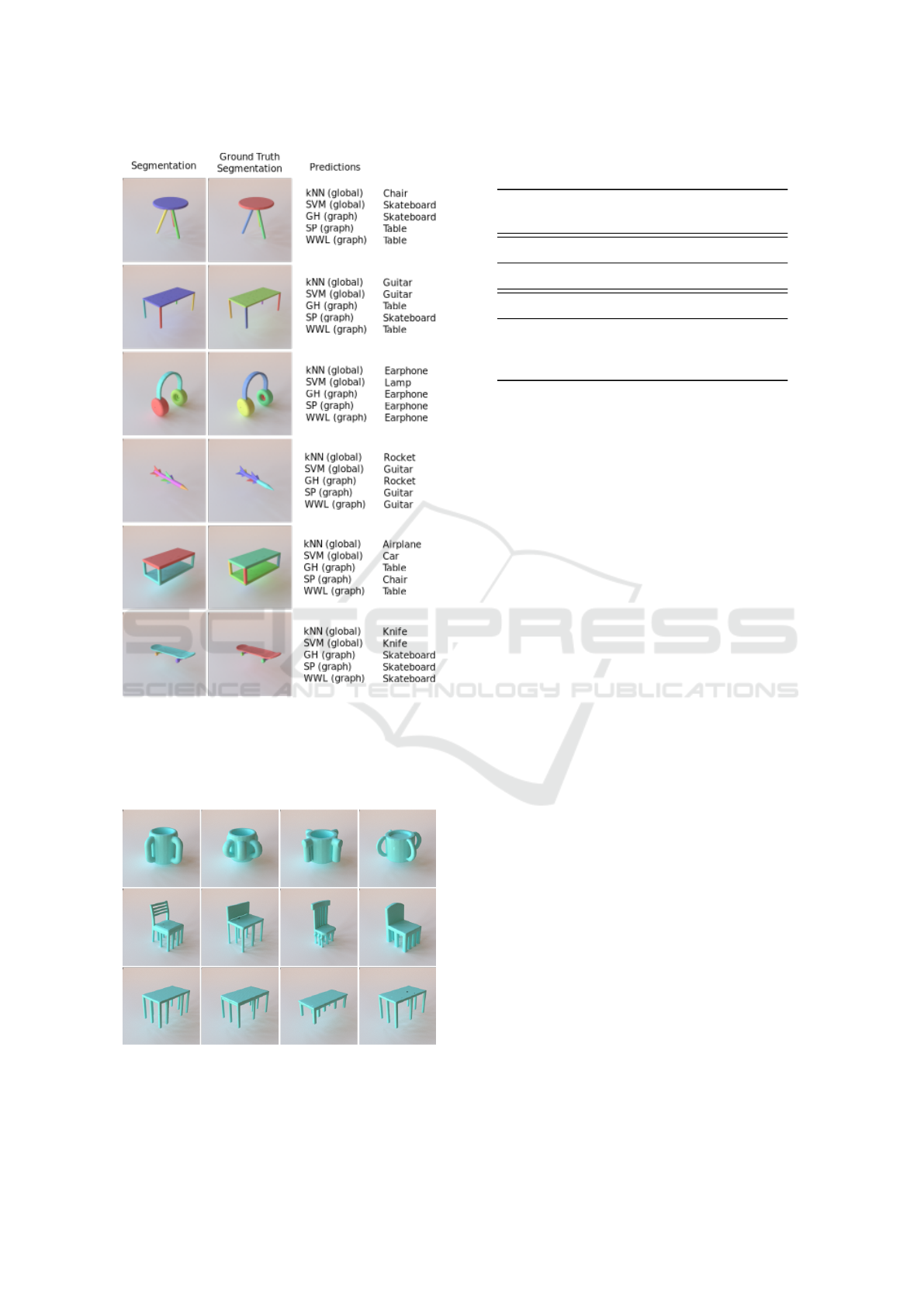
Figure 3: Qualitative classiﬁcation results of global clas-

siﬁers and graph classiﬁers based on automatic segmenta-

tions using the VFH descriptor. Groundtruth segmentation

is shown for comparison of segmentations. Note, GH, SP

and WWL predictions are based on automatic segmentation

from (Au et al., 2011), not groundtruth segmentations.

Figure 4: Artiﬁcial Object examples.

Table 2: Classiﬁcation accuracy of tested methods on artiﬁ-

cial objects. The columns refer to different descriptors.

Method VFH ESF Folding-

Net

Global descriptors

SVM 72 80 84

Graph-based

GH, autom. seg. 78 76 96

SP, autom. seg. 90 84 98

WWL, autom. seg. 76 88 98

ShortestPath on the FoldingNet descriptor. These re-

sults may indicate that the graph kernel methods make

better use of substructures in order to predict the ﬁnal

object classes. Thus, these graph kernel methods are

recommended to boost classiﬁcation performance.

6 CONCLUSIONS

This work investigated the utility of representing ob-

jects in terms of their substructures. To this end,

a comparison on three different graph kernels op-

erating on automatically extracted object parts was

conducted. Furthermore, three 3D feature extrac-

tors that describe these parts were analyzed regard-

ing their suitability for object classiﬁcation. A com-

parison against global (whole-object) descriptors sug-

gests that this part-based approach indeed improves

performance, especially if the Wasserstein Weisfeiler-

Lehman kernel is used. Our results on part graphs

using groundtruth segmentations indicate further po-

tential for improvement by making use of better seg-

mentation algorithm (as soon as this is available). We

conﬁrmed the ﬁnding of parts being useful with an

even stronger effect on a novel dataset of peculiar ob-

jects that deviate from standard object class concepts.

Since our approach comes with additional pro-

cessing steps (mesh cleanup, segmentation, individ-

ual descriptor extraction for each object part), the use

of this pipeline is recommended in cases where clas-

siﬁcation accuracy is required to be maximized and

additional computation cost is less critical.

REFERENCES

Achlioptas, P., Diamanti, O., Mitliagkas, I., and Guibas,

L. (2017). Representation learning and adversar-

ial generation of 3d point clouds. arXiv preprint

arXiv:1707.02392.

VISAPP 2021 - 16th International Conference on Computer Vision Theory and Applications

424

Au, O. K.-C., Zheng, Y., Chen, M., Xu, P., and Tai, C.-

L. (2011). Mesh segmentation with concavity-aware

ﬁelds. IEEE Transactions on Visualization and Com-

puter Graphics, 18(7):1125–1134.

Bay, H., Tuytelaars, T., and Van Gool, L. (2006). Surf:

Speeded up robust features. In Leonardis, A., Bischof,

H., and Pinz, A., editors, Computer Vision – ECCV

2006, pages 404–417, Berlin, Heidelberg. Springer

Berlin Heidelberg.

Biederman, I. (1987). Recognition-by-components: a the-

ory of human image understanding. Psychological re-

view, 94(2):115.

Borgwardt, K. M. and Kriegel, H.-P. (2005). Shortest-path

kernels on graphs. In Fifth IEEE International Confer-

ence on Data Mining (ICDM’05), pages 8–pp. IEEE.

Bronstein, A. M., Bronstein, M. M., Guibas, L. J., and Ovs-

janikov, M. (2011). Shape google: Geometric words

and expressions for invariant shape retrieval. ACM

Transactions on Graphics (TOG), 30(1):1–20.

Chang, A. X., Funkhouser, T. A., Guibas, L. J., Hanra-

han, P., Huang, Q., Li, Z., Savarese, S., Savva, M.,

Song, S., Su, H., Xiao, J., Yi, L., and Yu, F. (2015).

Shapenet: An information-rich 3d model repository.

CoRR, abs/1512.03012.

Chen, X., Golovinskiy, A., and Funkhouser, T. (2009). A

benchmark for 3D mesh segmentation. ACM Trans-

actions on Graphics (Proc. SIGGRAPH), 28(3).

Cortes, C. and Vapnik, V. (1995). Support-vector networks.

Machine learning, 20(3):273–297.

Fei-Fei, L. and Perona, P. (2005). A bayesian hierarchical

model for learning natural scene categories. In 2005

IEEE Computer Society Conference on Computer Vi-

sion and Pattern Recognition (CVPR’05), volume 2,

pages 524–531. IEEE.

Feragen, A., Kasenburg, N., Petersen, J., de Bruijne, M.,

and Borgwardt, K. (2013). Scalable kernels for graphs

with continuous attributes. In Advances in neural in-

formation processing systems, pages 216–224.

Floyd, R. W. (1962). Algorithm 97: shortest path. Commu-

nications of the ACM, 5(6):345.

George, D., Xie, X., and Tam, G. K. (2018). 3d mesh

segmentation via multi-branch 1d convolutional neu-

ral networks. Graphical Models, 96:1–10.

Golovinskiy, A. and Funkhouser, T. (2008). Randomized

cuts for 3d mesh analysis. In ACM SIGGRAPH Asia

2008 papers, pages 1–12. ACM New York, NY, USA.

Hanocka, R., Hertz, A., Fish, N., Giryes, R., Fleishman,

S., and Cohen-Or, D. (2019). Meshcnn: a network

with an edge. ACM Transactions on Graphics (TOG),

38(4):1–12.

Huang, J., Su, H., and Guibas, L. (2018). Robust water-

tight manifold surface generation method for shapenet

models. arXiv preprint arXiv:1802.01698.

Kalogerakis, E., Averkiou, M., Maji, S., and Chaudhuri, S.

(2017). 3d shape segmentation with projective convo-

lutional networks. In Proceedings of the IEEE Con-

ference on Computer Vision and Pattern Recognition,

pages 3779–3788.

Kalogerakis, E., Hertzmann, A., and Singh, K. (2010).

Learning 3d mesh segmentation and labeling. In ACM

SIGGRAPH 2010 papers, pages 1–12. Citeseer.

Kanezaki, A., Matsushita, Y., and Nishida, Y. (2018). Ro-

tationnet: Joint object categorization and pose estima-

tion using multiviews from unsupervised viewpoints.

In Proceedings of the IEEE Conference on Computer

Vision and Pattern Recognition, pages 5010–5019.

Kazhdan, M., Funkhouser, T., and Rusinkiewicz, S. (2003).

Rotation invariant spherical harmonic representation

of 3 d shape descriptors. In Symposium on geometry

processing, volume 6, pages 156–164.

Kipf, T. N. and Welling, M. (2016). Semi-supervised clas-

siﬁcation with graph convolutional networks. arXiv

preprint arXiv:1609.02907.

Kriege, N. M., Johansson, F. D., and Morris, C. (2020). A

survey on graph kernels. Applied Network Science,

5(1):1–42.

Le, T., Bui, G., and Duan, Y. (2017). A multi-view recurrent

neural network for 3d mesh segmentation. Computers

& Graphics, 66:103–112.

Li, J., Chen, B. M., and Lee, G. H. (2018). So-net: Self-

organizing network for point cloud analysis. arXiv

preprint arXiv:1803.04249.

Lien, J.-M. and Amato, N. M. (2007). Approximate con-

vex decomposition of polyhedra. In Proceedings of

the 2007 ACM symposium on Solid and physical mod-

eling, pages 121–131.

Loosli, G., Canu, S., and Ong, C. S. (2015). Learning svm

in kre

ın spaces. IEEE transactions on pattern analysis

and machine intelligence, 38(6):1204–1216.

Lowe, D. G. (1999). Object recognition from local scale-

invariant features. In Proceedings of the seventh

IEEE international conference on computer vision,

volume 2, pages 1150–1157. Ieee.

Maturana, D. and Scherer, S. (2015). Voxnet: A 3d con-

volutional neural network for real-time object recog-

nition. In 2015 IEEE/RSJ International Conference

on Intelligent Robots and Systems (IROS), pages 922–

928. IEEE.

Monti, F., Boscaini, D., Masci, J., Rodola, E., Svoboda, J.,

and Bronstein, M. M. (2017). Geometric deep learn-

ing on graphs and manifolds using mixture model

cnns. In Proceedings of the IEEE Conference on Com-

puter Vision and Pattern Recognition, pages 5115–

5124.

Qi, C. R., Su, H., Mo, K., and Guibas, L. J. (2017a). Point-

net: Deep learning on point sets for 3d classiﬁcation

and segmentation. In Proceedings of the IEEE Con-

ference on Computer Vision and Pattern Recognition,

pages 652–660.

Qi, C. R., Su, H., Nießner, M., Dai, A., Yan, M., and

Guibas, L. J. (2016). Volumetric and multi-view cnns

for object classiﬁcation on 3d data. In Proceedings of

the IEEE conference on computer vision and pattern

recognition, pages 5648–5656.

Qi, C. R., Yi, L., Su, H., and Guibas, L. J. (2017b). Point-

net++: Deep hierarchical feature learning on point sets

in a metric space.

3D Object Classiﬁcation via Part Graphs

425

Rusu, R. B., Blodow, N., and Beetz, M. (2009). Fast point

feature histograms (fpfh) for 3d registration. In 2009

IEEE international conference on robotics and au-

tomation, pages 3212–3217. IEEE.

Rusu, R. B., Bradski, G., Thibaux, R., and Hsu, J. (2010).

Fast 3d recognition and pose using the viewpoint

feature histogram. In 2010 IEEE/RSJ International

Conference on Intelligent Robots and Systems, pages

2155–2162. IEEE.

Rusu, R. B. and Cousins, S. (2011). 3d is here: Point cloud

library (pcl). In 2011 IEEE international conference

on robotics and automation, pages 1–4. IEEE.

Schoeler, M. and W

org

otter, F. (2015). Bootstrapping the

semantics of tools: Affordance analysis of real world

objects on a per-part basis. IEEE Transactions on

Cognitive and Developmental Systems, 8(2):84–98.

Shapira, L., Shamir, A., and Cohen-Or, D. (2008). Con-

sistent mesh partitioning and skeletonisation using

the shape diameter function. The Visual Computer,

24(4):249.

Shervashidze, N., Schweitzer, P., Leeuwen, E. J. v.,

Mehlhorn, K., and Borgwardt, K. M. (2011).

Weisfeiler-lehman graph kernels. Journal of Machine

Learning Research, 12(Sep):2539–2561.

Siglidis, G., Nikolentzos, G., Limnios, S., Giatsidis, C.,

Skianis, K., and Vazirgiannis, M. (2018). Grakel:

A graph kernel library in python. arXiv preprint

arXiv:1806.02193.

Sivic, J. and Zisserman, A. (2003). Video google: A text

retrieval approach to object matching in videos. In

null, page 1470. IEEE.

Su, H., Maji, S., Kalogerakis, E., and Learned-Miller, E.

(2015). Multi-view convolutional neural networks for

3d shape recognition. In Proceedings of the IEEE

international conference on computer vision, pages

945–953.

Togninalli, M., Ghisu, E., Llinares-L

opez, F., Rieck, B., and

Borgwardt, K. (2019). Wasserstein weisfeiler-lehman

graph kernels. In Advances in Neural Information

Processing Systems, pages 6436–6446.

Tombari, F., Salti, S., and Di Stefano, L. (2010). Unique sig-

natures of histograms for local surface description. In

European conference on computer vision, pages 356–

369. Springer.

Vaserstein, L. N. (1969). Markov processes over denumer-

able products of spaces, describing large systems of

automata. Problemy Peredachi Informatsii, 5(3):64–

72.

Wang, C., Pelillo, M., and Siddiqi, K. (2019a). Dominant

set clustering and pooling for multi-view 3d object

recognition. arXiv preprint arXiv:1906.01592.

Wang, Y., Sun, Y., Liu, Z., Sarma, S. E., Bronstein, M. M.,

and Solomon, J. M. (2019b). Dynamic graph cnn

for learning on point clouds. ACM Transactions on

Graphics (TOG), 38(5):1–12.

Wohlkinger, W. and Vincze, M. (2011). Ensemble of shape

functions for 3d object classiﬁcation. In 2011 IEEE

international conference on robotics and biomimetics,

pages 2987–2992. IEEE.

Wu, J., Zhang, C., Xue, T., Freeman, B., and Tenenbaum,

J. (2016). Learning a probabilistic latent space of ob-

ject shapes via 3d generative-adversarial modeling. In

Advances in neural information processing systems,

pages 82–90.

Wu, Z., Song, S., Khosla, A., Yu, F., Zhang, L., Tang, X.,

and Xiao, J. (2015). 3d shapenets: A deep representa-

tion for volumetric shapes. In Proceedings of the IEEE

conference on computer vision and pattern recogni-

tion, pages 1912–1920.

Yang, Y., Feng, C., Shen, Y., and Tian, D. (2017). Fold-

ingnet: Interpretable unsupervised learning on 3d

point clouds. CoRR, abs/1712.07262.

Yi, L., Kim, V. G., Ceylan, D., Shen, I.-C., Yan, M., Su, H.,

Lu, C., Huang, Q., Sheffer, A., and Guibas, L. (2016).

A scalable active framework for region annotation in

3d shape collections. SIGGRAPH Asia.

Yu, T., Meng, J., and Yuan, J. (2018). Multi-view harmo-

nized bilinear network for 3d object recognition. In

Proceedings of the IEEE Conference on Computer Vi-

sion and Pattern Recognition, pages 186–194.

VISAPP 2021 - 16th International Conference on Computer Vision Theory and Applications

426