Developing a Machine Learning Workﬂow to Explain Black-box Models

for Alzheimer’s Disease Classiﬁcation

Louise Bloch

1,2 a

and Christoph M. Friedrich

1,2 b

1

Department of Computer Science, University of Applied Sciences and Arts Dortmund,

Emil-Figge-Str. 42, 44227 Dortmund, Germany

2

Institute for Medical Informatics, Biometry and Epidemiology (IMIBE), University Hospital Essen, Essen, Germany

Keywords:

Interpretable Machine Learning, Alzheimer’s Disease Classiﬁcation, Shapley Values, Alzheimer’s Disease

Neuroimaging Initiative, Australian Imaging and Lifestyle Flagship Study of Ageing.

Abstract:

Many research articles used difﬁcult-to-interpret black-box Machine Learning (ML) models to classify

Alzheimer’s disease (AD) without examining their biological relevance. In this article, an ML workﬂow was

developed to interpret black-box models based on Shapley values. This workﬂow enabled the model-agnostic

visualization of complex relationships between model features and predictions and also the explanation of

individual predictions, which is important in clinical practice. To demonstrate this workﬂow, eXtreme Gradi-

ent Boosting (XGBoost) and Random Forest (RF) classiﬁers were trained for AD classiﬁcation. All models

were trained on the Alzheimer’s Disease Neuroimaging Initiative (ADNI) or Australian Imaging and Lifestyle

ﬂagship study of Ageing (AIBL) dataset and were validated for independent test datasets of both cohorts. The

results showed improved performances for black-box models in comparison to simple Classiﬁcation and Re-

gression Trees (CARTs). For the classiﬁcation of Mild Cognitive Impairment (MCI) conversion and the ADNI

training dataset, the best model achieved a classiﬁcation accuracy of 71.03 % for the ADNI test dataset and

67.65 % for the entire AIBL dataset. This RF used a logical long-term memory test, the count of Apolipopro-

tein E ε4 (ApoEε4) alleles and the volume of the left hippocampus as the most important features.

1 INTRODUCTION

Alzheimer’s Disease (AD) is a neurodegenerative

disease (Alzheimer’s Association, 2020), the most

frequent cause of dementia and a globally grow-

ing health problem (Patterson, 2018). Small brain

changes begin decades before clinical symptoms were

noted (Lloret et al., 2019). The early identiﬁcation of

patients at risk is important to recruit and monitor sub-

jects for therapy studies as there currently is no causal

therapy (Alzheimer’s Association, 2020). Many ap-

proaches investigated the early AD diagnosis using

Machine Learning (ML). Some approaches used in-

terpretable models like Decision Trees (DTs) or logis-

tic regression to investigate general associations (Li

et al., 2020; Mofrad et al., 2018). However, black-

box models like eXtreme Gradient Boosting (XG-

Boost) (Chen and Guestrin, 2016), Random Forests

(RF) (Breiman, 2001) or Convolutional Neural Net-

works (CNNs) (LeCun et al., 2015) often achieved

a

https://orcid.org/0000-0001-7540-4980

b

https://orcid.org/0000-0001-7906-0038

improved performances (Bloch and Friedrich, 2019;

Grassi et al., 2019) but were challenging to interpret.

Moreover, most AD ML models lacked for external

validation (Samper-Gonz

´

alez et al., 2018).

Interpretable ML was developed to explain black-

box models. This is relevant in AD as it was not com-

pletely understood yet. Additionally, interpretable

ML enables the inspection of the biological relevance

of black-box ML models. There have been some ar-

ticles using interpretable ML in AD diagnosis. For

example, (Pelka et al., 2020) trained Long Short-

Term Memory (LSTM) (Hochreiter and Schmidhu-

ber, 1997) based Recurrent Neural Networks (RNN)

(Rumelhart et al., 1986) to classify Cognitive Normal

(CN) vs. Mild Cognitive Impaired (MCI) subjects.

The paper compared different techniques to fuse so-

ciodemographic and genetic data with Magnetic Res-

onance Imaging (MRI). The models were evaluated

for an AD subset (Dlugaj et al., 2010) of the Heinz

Nixdorf Risk Factors Evaluation of Coronary Calci-

ﬁcation and Lifestyle (RECALL) (HNR) (Schmer-

mund et al., 2002) (61 MCI and 59 CN) and the

Bloch, L. and Friedrich, C.

Developing a Machine Learning Workﬂow to Explain Black-box Models for Alzheimer’s Disease Classiﬁcation.

DOI: 10.5220/0010211300870099

In Proceedings of the 14th International Joint Conference on Biomedical Engineering Systems and Technologies (BIOSTEC 2021) - Volume 5: HEALTHINF, pages 87-99

ISBN: 978-989-758-490-9

Copyright

c

87

Alzheimer’s Disease Neuroimaging Initiative (ADNI)

(Petersen et al., 2010) study (397 MCI and 227 CN).

Gradient-weighted Class Activation Mapping (Grad-

CAM) (Selvaraju et al., 2017) was used to visually ex-

plain individual model decisions. Initial observations

showed a focus on biologically plausible regions.

(Das et al., 2019) presented a new interpretable

model, based on distinct weighted rules. The model

was evaluated for 151 subjects of the ADNI cohort

(97 AD and 54 CN). The framework was trained in

two stages, the ﬁrst stage used plasma features to train

the interpretable model. Subjects with an unclear pre-

diction were propagated to the second stage, where a

Support Vector Machine (SVM) (Cortes and Vapnik,

1995) was trained using invasive Cerebrospinal Fluid

(CSF) markers. The evaluation included both, Cross-

Validation (CV) and an independent test dataset. For

the test dataset an Area Under the Receiver Operating

characteristics Curve (AUC) of 0.81 was reached.

(Hammond et al., 2020) used RF feature im-

portance to examine the predictive inﬂuence of β-

amyloid plaques, tau tangles and neurodegeneration

during the disease progress. The experiments were

performed for 405 ADNI subjects (148 CN, 147

MCI and 110 AD). β-amyloid Positron Emission

Tomography (PET) was used to detect β-amyloid

plaques, invasive CSF features surrogated tau-tangles

and MRI and Fluorodeoxyglucose (FDG) PET scans

were used to determine neurodegeneration. Models

trained to classify the early AD stages preferred fea-

tures representing tau tangles and β-amyloid-plaques,

whereas models for later stage classiﬁcation favoured

surrogates for neurodegeneration. The observations

were reproduced using SHapley Additive exPlana-

tions (SHAP) (Lundberg and Lee, 2017) and Gradient

Tree Boosting (GTB) (Friedman, 2001). The RF clas-

siﬁer and the entire feature set reached accuracies of

73.17 %, 71.01 %, and 90.34 % for the CN vs. MCI,

MCI vs. AD, and CN vs. AD classiﬁcations.

(Rieke et al., 2018) compared the four heatmap

visualisation methods sensitivity analysis (Simonyan

et al., 2014), guided backpropagation (Springenberg

et al., 2015), occlusion (Zeiler and Fergus, 2014) and

brain area occlusion inspired by (Yang et al., 2018) for

3D-CNNs. The CNN model was trained using 969

MRI scans of 344 ADNI subjects (151 CN and 193

AD). It is important to ensure independent training

and test datasets if multiple scans per subject were

used (Wen et al., 2020) which was unclear for this

article. Thus, the CV accuracy of 77 % ± 6 %, was

questionable. The heatmaps of all the methods were

focused on AD-related anatomical brain areas.

(Wang et al., 2019) introduced an interpretable

deep learning model, consisting of a Generative Ad-

versarial Network (GAN) (Goodfellow et al., 2014)

to extend the training dataset, a regression network

to generate feature vectors from adjacent visits and

a classiﬁcation model. The regression model itera-

tively estimated the feature vector at a prospective

visit and the classiﬁcation model does the ﬁnal pre-

diction. Longitudinal volumetric MRI features were

used to classify 101 progressive MCI (pMCI) vs. 115

stable MCI (sMCI) ADNI subjects. The model out-

performed SVMs and artiﬁcial neural networks.

In this article, an ML workﬂow was developed, to

interpret black-box models based on model-agnostic

Shapley values. In comparison to classical feature im-

portance methods, the advantage was to obtain an in-

dividual explanation for each subject and to observe

complex relationships between the features and the

prediction. The workﬂow was evaluated by train-

ing XGBoost and RF models to inspect different AD

stages but was not limited to those models. Two

different cohorts were used for model training, the

ADNI and the Australian Imaging and Lifestyle ﬂag-

ship study of Ageing (AIBL) (Ellis et al., 2009). Each

model was trained on one cohort and evaluated for the

independent test datasets of both cohorts. The train-

ing has been performed for two different non-invasive

feature sets. Section 2 describes the datasets and in-

terpretation methods. The ML workﬂow is delineated

in Section 3. The experimental results are explained

in Section 4. Section 5 ﬁnally discusses the results

and gives an outlook about future work.

2 MATERIALS AND METHODS

2.1 Dataset

Data used in the preparation of this article were ob-

tained from the ADNI (Petersen et al., 2010) and

the AIBL (Ellis et al., 2009) cohorts. The datasets

included 1700 ADNI and 612 AIBL subjects. The

ADNI dataset consisted of 512 CN, 853 MCI and

335 AD subjects. The MCI subjects were split into

two subsets. 401 Baseline (BL) MCI subjects had

no diagnostic changes in all visits and were classi-

ﬁed as sMCI subjects. 319 BL MCI subjects con-

verted to AD at subsequent visits and were classiﬁed

as pMCI. BL MCI subjects, who reverted to CN for

at least one visit, pMCI subjects who reverted to MCI

and subjects with no follow-up diagnosis assigned to

none of these two classes. ADNI subjects from the

study phases ADNI-1 (809 subjects), ADNIGO (127

subjects) and ADNI-2 (764 subjects) were included.

The time between the BL and the ﬁnal diagnosis for

sMCI and pMCI subjects ranged between 4.7 and

HEALTHINF 2021 - 14th International Conference on Health Informatics

88

Table 1: ADNI demographics at BL. The mean and standard deviation are given for all continuous variables.

n Age (in years) Gender/ females (in %) MMSE CDR ApoEε4 (0/1/2) (in %)

CN 512 74.2±5.8 51.8 29.1±1.1 0.0±0.0 (71.3 / 26.2 / 2.3)

MCI 853 73.1±7.6 40.8 27.6±1.8 0.5±0.0 (49.4 / 39.5 / 10.8)

sMCI 401 73.2±7.5 40.4 27.8±1.8 0.5±0.0 (56.9 / 33.9 / 9.2)

pMCI 319 74.0±7.1 40.1 27.0±1.7 0.5±0.0 (34.2 / 49.5 / 16.3)

AD 335 75.0±7.8 44.8 23.2±2.1 0.8±0.3 (33.1 / 47.2 / 19.1)

Σ 1700 73.8±7.2 44.9 27.2±2.7 0.4±0.3 (52.8 / 37.0 / 9.9)

156.2 months. The same inclusion criteria were ap-

plied to the AIBL cohort. This resulted in 447 CN,

94 MCI, 16 sMCI, 18 pMCI and 71 AD subjects and

the time between the BL and the ﬁnal diagnosis for

sMCI and pMCI subjects ranged between 16.9 and

55.1 months. The demographic data of the ADNI and

AIBL datasets are summarized in Tables 1 and 2.

For each subject, the BL 1.5 T or 3 T T1-weighted

Magnetization-Prepared Rapid Gradient-Echo (MP-

RAGE) MRI scan was selected. In this study, fully

preprocessed ADNI scans (Jack et al., 2015) were

used. There are no preprocessed AIBL MRI scans

available, thus unprocessed scans were used. Volu-

metric features were extracted from the MRI scans

using FreeSurfer v6.0 (Fischl, 2012). Volumetric

features of 34 cortical areas per hemisphere of the

Desikan-Killiany atlas (Desikan et al., 2006), 34 sub-

cortical areas (Fischl et al., 2002) and the estimated

Total Intracranial Volume (eTIV) were extracted. The

volumetric features were normalized by eTIV as rec-

ommended for volumes in (Westman et al., 2012).

The experiments were performed using two fea-

ture sets. Feature Set 1 (FS1) included 103 MRI fea-

tures, age, gender and count of Apolipoprotein E ε4

(ApoEε4) alleles (106 features). Gender and ApoEε4

were coded as two and three binary dummy variables.

APOE4.X (X∈{0,1,2}) indicated if a subject had X

ApoEε4 alleles. PTGENDER.MALE speciﬁes if the

subject was male and PTGENDER.FEMALE if it was

female. All dummy variables had a value of one, if

the expression is true, and zero otherwise. In Feature

Set 2 (FS2) Mini-Mental State Examination (MMSE),

Clinical Dementia Rating (CDR), and logical tests

to evaluate the long-term (Logical memory, delayed

(LDELTOTAL)) and the short-term memory (Logical

memory, immediate (LIMMTOTAL)) were added to

FS1 (110 features). The CDR score was excluded for

sMCI vs. pMCI classiﬁcation due to small variance.

2.2 Interpretable ML

An overview of different methods to interpret ML

models can be found in (Molnar, 2019). Some mod-

els like DTs and logistic regression models are in-

terpretable by design. However, the interpretation

of black-box models, which often achieve better re-

sults, is more complicated. This article used model-

agnostic Shapley values. In contrast to the model-

speciﬁc approaches, it is suitable to explain any type

of ML model, and enabled comparability. Addition-

ally, Shapley values are local models, which explain

individual observations and thus achieve a high clini-

cal beneﬁt and good performances.

2.2.1 Shapley Values

Shapley values (Shapley, 1953) are afﬁliated to coali-

tion game theory. The aim is to determine the effect

of a single feature of an observation on the overall

prediction. Shapley values explain the differences be-

tween the average model prediction and the prediction

of an observation by different features. Thus, Shap-

ley values are based on the additive linear explanation

model shown in equation 1. The model prediction

f (x) of an observation x is explained by the feature

effects Φ

j

and the average model prediction Φ

0

. x

0

is

a simpliﬁed representation of the observation x. For

tabular data, this is a binned binary feature represen-

tation. N is the number of simpliﬁed features.

f (x) = Φ

0

+

N

∑

j=1

Φ

j

x

0

j

(1)

Shapley values explain the overall prediction of an ob-

servation by fairly distributed feature effects. There-

fore, they are deﬁned as the average contribution of

a feature expression for the prediction in all subsets,

described in equation 2. To calculate the Shapley

value Φ

i

of a feature i and an observation, it was re-

quired to determine all subsets S of the entire feature

set F. It was necessary to retrain and evaluate the

black-box model f

S

(S) for each subset S. The differ-

ences in model performance trained with ( f

S∪i

(S ∪ i))

and without ( f

S

(S)) the feature at interest i were cal-

culated. The Shapley value is the weighted average

difference of all subsets. The weights depend on the

total number of model features |F| and the number of

feature expressions |S| in the subset S. High weights

were assigned to both, subsets with few and with

many features, to support the estimation of the main

individual effects and the total effects.

Developing a Machine Learning Workﬂow to Explain Black-box Models for Alzheimer’s Disease Classiﬁcation

89

Table 2: AIBL demographics at BL. The mean and standard deviation are given for all continuous variables.

n Age (in years) Gender/ females (in %) MMSE CDR ApoEε4 (0/1/2) (in %)

CN 447 72.5±6.2 57.0 28.7±1.2 0.0±0.1 (70.7 / 26.4 / 2.9)

MCI 94 75.3±7.0 46.8 27.1±2.2 0.5±0.1 (51.1 / 37.2 / 11.7)

sMCI 16 76.4±7.7 50.0 27.6±2.4 0.5±0.0 (56.2 / 37.5 / 6.2)

pMCI 18 78.0±7.1 50.0 26.8±2.0 0.5±0.0 (16.7 / 66.7 / 16.7)

AD 71 73.3±7.9 59.2 20.5±5.7 0.9±0.6 (32.4 / 49.3 / 18.3)

Σ 612 73.0±6.6 55.7 27.5±3.5 0.2±0.4 (63.2 / 30.7 / 6.0)

Φ

i

=

∑

S⊆F\{i}

|S|!(|F| − |S| −1)!

|F|!



f

S∪{i}

(S∪i)− f

S

(S)



(2)

The computational effort for the exact calculation of

Shapley values increases exponentially with the num-

ber of features. In this paper, Shapley sampling values

(

ˇ

Strumbelj and Kononenko, 2013) which are based on

Monte-Carlo sampling estimated the Shapley values

to avoid time-consuming repeated training and eval-

uation. The estimation of a Shapley value

b

Φ

i

(x) for

a feature i and an observation x is demonstrated in

equation 3. M is the number of Monte-Carlo simu-

lations and x

m

±i

is the observation x with some feature

expressions replaced by random values. In each simu-

lation, x

m

+i

and x

m

−i

are identical, except that the feature

i was randomly replaced in x

m

−i

and not in x

m

+i

. f is the

black-box model. Each Shapley sampling value is the

mean of the differences of M samples.

b

Φ

i

(x) =

1

M

∑

m=1



f (x

m

+i

) − f (x

m

−i

)



(3)

3 ML WORKFLOW

The ML workﬂow, shown in Figure 1 and im-

plemented using the programming language R ver-

sion 3.5.3 (R Core Team, 2019), allows the interpreta-

tion of black-box models trained to classify early AD.

Subject and feature selection and image process-

ing are described in Section 2.1. Feature fusion was

performed by a concatenation. The dataset was dis-

tinctly split into an 80 % training and a 20 % test

dataset. This split was performed within the diagnosis

groups. Model training, hyperparameter tuning and

model interpretation was carried out for the training

dataset and the performance evaluation was executed

for the independent test datasets of both cohorts.

3.1 Hyperparameter Tuning

Bayesian optimization (Mo

ˇ

ckus, 1975) was imple-

mented using the R package rBayesianOptimization

version 1.1.0 (Yan, 2016) to tune the model hyper-

parameters. The idea is, to model the dependency

of the hyperparameters and the model performance

by a Gaussian Process (GP). Ten nearly random ini-

tial parameters were deﬁned by a Latin hypercube

design (LHD) (McKay et al., 1979), which was im-

plemented using the R package SPOT version 2.0.3

(Bartz-Beielstein et al., 2005). The range of each

parameter was split into ten intervals to randomly

choose one sample per interval. The resulting ten

samples per parameter were randomly matched across

the parameters.

The ML model was evaluated for these combi-

nations using 10 × 10-fold CV (Refaeilzadeh et al.,

2009) to estimate the model performance for the test

dataset using the hyperparameters. 10 × 10-fold CV

was implemented by splitting the training dataset

into ten distinct folds using the R package caret ver-

sion 6.0-82 (Kuhn, 2019). The splits were executed

separately for each diagnosis. Ten iterations were per-

formed, each with a different fold used as validation

dataset (10 %). The training dataset included the re-

maining nine folds (90 %). This procedure was re-

peated for ten times, with shufﬂed data in each run.

The GP was ﬁtted to predict the average CV ac-

curacy for the initial parameter combinations. After-

wards, the model was optimized to choose the next

parameter combination. Here, the Upper Conﬁdence

Bounds (UCB) acquisition function (equation 4) was

used. ˆµ

Θ

is the performance estimation of the GP and

ˆ

Σ

Θ

is the covariance at parameter combination Θ. κ

weights the inﬂuence of exploitation and exploration

during the optimization. A high κ-value preferred ex-

ploration and small values favour exploitation. All

experiments used the default value of 2.576.

UCB(Θ) = ˆµ

Θ

+ κ ·

ˆ

Σ

Θ

(4)

Iteratively, the new hyperparameter combination was

evaluated using CV and the results were added to re-

ﬁne the GP and to determine a new combination. This

procedure was repeated 25 times. The best combina-

tion was chosen to train the ﬁnal model.

HEALTHINF 2021 - 14th International Conference on Health Informatics

90

Final model generation

Volume

calculation

SegmentationRegistration

Pre-

processing

Hyperparameter tuning

Evaluation

Image processing

Data

splitting

Subject

selection

Model

training

Resampling

Pre-

processing

Model

training

Pre-

processing

Test dataset

Training

dataset

Initialize

parameter

combinations

Determine promising

parameter combination

Determine

best

parameter

combination

Met exit

condition

Continue

parameter tuning

Feature

selection

MRI scan

selection

Feature

fusion

Generate

interpretation

model

Training cohort

Training and

External

Validation

cohort

Figure 1: ML workﬂow.

Table 3: XGBoost hyperparameters and intervals.

Name Minimum Maximum

nrounds 1 500

eta 0 1

gamma 0 20

max depth 1 20

min child weights 1 30

subsample 0 1

colsample bytree 0 1

3.2 Model Training

The preprocessing included centering, scaling, me-

dian imputation and Synthetic Minority Over-

sampling Technique (SMOTE) (Chawla et al., 2002)

to compensate class imbalances. It was implemented

using the R package caret version 6.0-82 (Kuhn,

2019). Afterwards, the ML models were trained.

XGBoost (Chen and Guestrin, 2016) is an im-

plementation of gradient boosting (Friedman, 2001),

distributed as an open-source software library. The

idea of boosting algorithms is, to iteratively combine

multiple weak classiﬁers to get a strong joint clas-

siﬁer. Gradient boosting meets this assumption by

learning the gradients of the previous classiﬁer. The

sum of the weak classiﬁer results is the ﬁnal predic-

tion. The main advantages of XGBoost are scalability,

parallelization and distributed execution. The XG-

Boost hyperparameters are summarized in Table 3.

nrounds sets the number of boosting iterations and

eta was the learning rate, which controls the prefer-

ence of classiﬁers at early iterations. The minimum

loss reduction required to split a node is deﬁned by

gamma, max depth sets the maximum tree depth and

min child weights was the minimum number of ob-

servations in a child node. subsample and colsam-

ple bytree set the proportion of randomly subsampled

training instances and features per iteration. An XG-

Boost tree classiﬁer was implemented using the R

package xgboost version 0.82.1 (Chen et al., 2019).

RF (Breiman, 2001) is an ensemble black-box

Table 4: RF hyperparameters and optimization intervals.

Name Minimum Maximum

mtry 2 # features

ntree 250 1250

nodesize 1 30

maxnodes 50 100

model based on multiple DTs and was implemented

using the R package randomForest version 4.6-14

(Liaw and Wiener, 2002). Each DT was trained us-

ing randomly chosen features and bootstrap sampling

(Efron and Tibshirani, 1986) of the training dataset.

The results of the DTs were ﬁnally summarized using

a majority voting. The hyperparameter ntree sets the

number of DTs. Each split considered a random sub-

set of mtry features. The minimum size of leaf nodes

was deﬁned by nodesize and maxnodes determines the

maximum number of leaf nodes per DT. Table 4 sum-

marizes the RF hyperparameters.

Classiﬁcation and Regression Trees (CARTs)

(Breiman et al., 1984) were chosen as interpretable

models and implemented using the R package rpart

version 4.1-13 (Therneau and Atkinson, 2018). Dur-

ing the training of CARTs, successively decision rules

of the form x ≤ t for numerical or x ∈ t for categorical

features were learned with t as a threshold or a subset.

Each possible split was ranked by the Gini-coefﬁcient

(equation 5) to ﬁnd the best rule. In this equation, c is

the total number of classes and p(i), is the proportion

of observations of class i in a node.

f (p) =

c

∑

i=1

p(i) ·



1 − p(i)



(5)

This method was iteratively repeated as long as no

split with a minimum improvement of the complexity

parameter cp can be performed. This hyperparameter

was tuned in a range between 0 and 1.

Developing a Machine Learning Workﬂow to Explain Black-box Models for Alzheimer’s Disease Classiﬁcation

91

3.3 Interpretation Model

Shapley sampling values were implemented using the

R package fastshap version 0.0.5 (Greenwell, 2020)

to explain the black-box models. All experiments per-

formed 5000 Monte-Carlo simulations to estimate the

Shapley values. The SHAP force plot in Figure 3 ex-

plains the model prediction of an individual observa-

tion. The plot shows, that the individual prediction

consists of the sum of all feature Shapley values and

the average model prediction. Feature expressions

with high positive Shapley values had a strong pos-

itive effect on the prediction and small negative Shap-

ley values represent small negative effects.

SHAP summary plots (Lundberg et al., 2018) ex-

plain the model results for the entire training dataset.

Each point shows a Shapley value for a subject and a

feature and is colored depending on the feature value.

The vertical axis represented the features, ordered by

the mean absolute Shapley values, and their distribu-

tion. The plots were limited to the top ten features.

4 RESULTS

The results of the experiments with FS1 and FS2 are

summarized in Tables 5 and 6. For both feature sets,

the best results were achieved for CN vs. AD clas-

siﬁcation. For example, a perfect CV accuracy was

achieved by training an RF with FS2 of the ADNI

dataset. The CART, trained with FS2 of the ADNI

dataset, reached a perfect classiﬁcation for the ADNI

test dataset. The best accuracy for the AIBL test

dataset was 99.05 % and was achieved by training an

XGBoost model with FS2 of the AIBL dataset.

Only 16 sMCI and 18 pMCI AIBL subjects were

selected, thus, AIBL was only used for external vali-

dation in this case. For FS1 and FS2 the RF achieved

the best results to classify MCI conversion. The FS2

model yielded an accuracy of 71.03 % for the inde-

pendent ADNI and 67.65 % for the AIBL test dataset.

For FS1, accuracies of 68.28 % for the ADNI and

79.41 % for the AIBL test datasets were reached.

4.1 Feature Set 1 vs. Feature Set 2

In general, the performances reached with FS2 (Ta-

ble 6) outperformed the results achieved with FS1

(Table 5). Adding cognitive test results to FS1 im-

proved the distinction of the BL diagnoses. Minor im-

provements were noted for the MCI conversion pre-

diction. For example, the RF trained with FS2 for

MCI conversion prediction outperformed the model

trained with FS1 by 2.75 % for the ADNI test dataset

●

●●

●

● ●

●

●●

●

● ●

●

●●

●

●●

●

● ●

●

●●

●

●●

●

●●

●

●●

●

●●

●

● ●

●

● ●

●

●●

●

● ●

●

●●

●

●●

●

●●

●

● ●

●

●●

●

● ●

●

●●

●

●●

●

● ●

●

lh_inferiorparietal_volume

lh_middletemporal_volume

Right.Hippocampus

rh_entorhinal_volume

Right.Inf.Lat.Vent

APOE4.1

Right.Amygdala

Left.Amygdala

Left.Hippocampus

APOE4.0

LDELTOTAL

−0.10 −0.05 0.00 0.05 0.10

Shapley value

Feature

Low High

Feature value

Figure 2: SHAP summary plot of the RF trained with ADNI

and FS2 for sMCI (0) vs. pMCI (1). APOE4.X (X∈{0,1,2})

indicates if a subject had X ApoEε4 alleles. A value of 1

(purple) indicates a true expression, and 0 (yellow) a false.

but for the AIBL dataset the FS1 model performed

11.76 % better.

Figure 2 shows a SHAP summary plot of the

RF trained with FS2. The most important feature

of this model was the LDELTOTAL cognitive test

score. Small LDELTOTAL scores, exhibited high

Shapley values, thus the model identiﬁed subjects

with small LDELTOTAL scores as pMCI subjects. It

was detected, that subjects with no ApoEε4 alleles

(APOE4.0 = 1) were more likely classiﬁed as sMCI

as subjects with one or two alleles (APOE4.0 = 0).

Consistently, the presence of a single ApoEε4 allele

(APOE4.1 = 1) was associated with pMCI subjects.

The two most important MRI features of this model

were the volumes of the left hippocampus and the left

amygdala. For both features, high values predomi-

nantly have Shapley values smaller zero and were thus

associated with sMCI subjects. The other MRI fea-

tures consistently show biologically plausible associ-

ations, corresponding to AD neurodegeneration (De-

Ture and Dickson, 2019).

Figure 3 shows a SHAP force plot of this model

to explain the individual prediction of an ADNI pMCI

subject. SHAP force plots are helpful to present in-

dividual contributions for clinical observations. The

Shapley values are visualized as arrows to explain

the differences between the average model prediction

(0.395) and the prediction of the individual observa-

tion (0.61). Here, the individual prediction was the

probability of the subject of being classiﬁed as pMCI.

The length of an arrow indicated the Shapley value.

Feature expressions with high Shapley values like the

LDELTOTAL score were visualized with long arrows.

Pathogenic feature expressions were colored in red.

For example, a small normalized feature expression

of 0.09 was measured for LDELTOTAL. This expres-

sion had the highest positive Shapley value of 0.034

to explain the overall prediction. Protective feature

HEALTHINF 2021 - 14th International Conference on Health Informatics

92

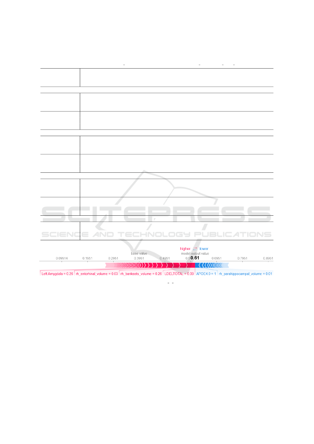
Table 5: Classiﬁcation results and hyperparameters for FS1. Comparison of CART, RF and XGBoost models trained on

ADNI and AIBL datasets. The best results in each section are highlighted in bold. Hyperparameters: CART: (cp), RF: (mtry,

ntree, nodesize, maxnodes), XGBoost: (max depth, nrounds, eta, gamma, colsample bytree, min child weight, subsample).

Model Trai-

ning

dataset

Hyperparameters CV accuracy

(mean±sd)

in %

Accuracy

test dataset

ADNI in %

Accuracy

test dataset

AIBL in %

CN vs. AD: No information rate test dataset: ADNI: 60.59, AIBL: 85.71

CART ADNI (0.013) 82.62±4.42 81.76 89.52

RF ADNI (27, 735, 1, 92) 88.14±4.05 90.00 88.57

XGBoost ADNI (2, 417, 0.120, 0.371, 0.349, 17.08, 0.746) 88.82±4.04 90.59 88.57

CART AIBL (0.803) 86.45±1.06 60.59 85.71

RF AIBL (1, 707, 9, 69) 89.27±5.19 83.53 95.24

XGBoost AIBL (1, 297, 0.246, 0.237, 0.436, 2.158, 0.732) 87.99±4.96 81.76 91.43

MCI vs. AD: No information rate test dataset: ADNI: 71.85, AIBL: 55.88

CART ADNI (0.441) 71.79±0.33 71.85 55.88

RF ADNI (10, 1250, 20, 100) 73.11±4.28 78.15 58.82

XGBoost ADNI (19, 259, 0.088, 9.922, 0.696, 19.255, 0.595) 72.42±4.12 75.63 55.88

CART AIBL (0.207) 58.42±13.58 57.14 55.88

RF AIBL (1, 1250, 7, 89) 71.93±12.22 66.81 70.59

XGBoost AIBL (19, 259, 0.088, 9.922, 0.696, 19.255, 0.595) 64.36±12.41 68.91 70.59

CN vs. MCI: No information rate test dataset: ADNI: 62.41, AIBL: 82.57

CART ADNI (0.028) 65.80±4.31 63.87 44.18

RF ADNI (23, 1250, 1, 100) 69.49±4.20 67.52 48.62

XGBoost ADNI (2, 417, 0.120, 0.371, 0.349, 17.080, 0.746) 68.89±4.07 68.98 40.37

CART AIBL (0.545) 82.65±0.96 37.59 82.57

RF AIBL (1, 1250, 20, 50) 79.91±4.59 55.84 83.49

XGBoost AIBL (2, 500, 0.109, 12.111, 1.000, 30.000, 0.157) 82.65±0.95 37.59 82.57

sMCI vs. pMCI: No information rate test dataset: ADNI: 55.86, entire AIBL dataset: 52.94

CART ADNI (0.063) 65.26±5.97 63.45 70.59

RF ADNI (17, 250, 18, 50) 67.94±5.49 68.28 79.41

XGBoost ADNI (2, 417, 0.120, 0.371, 0.349, 17.080, 0.746) 67.18±5.10 64.83 64.71

Figure 3: SHAP force plot for an ADNI pMCI subject (PTID = 123 S 0050) to explain the prediction of the RF trained with

ADNI and FS2 for sMCI (0) vs. pMCI (1). The arrow length indicates a Shapley value of the feature expression. Pathogenic

feature expressions are shown as red and protective expressions as blue arrows. The normalized feature expressions with the

highest absolute Shapley values are explained below the arrows. Mean prediction value (base value): 0.395. ApoEε4 and

gender were dummy coded (e.g. APOE4.0 = 1 means, that the subject had no ApoEε4 alleles).

expressions were colored in blue. In this plot, the ab-

sence of ApoEε4 alleles (APOE4.0 = 1) had a protec-

tive inﬂuence (Shapley value of -0.020) on the overall

prediction. The individual diagnosis of the subject at

interest was based on a large number of feature ex-

pressions and the most important ones are named in

the ﬁgure below the arrows.

The largest differences between the results of FS1

and FS2 were observed for the CN vs. MCI classiﬁ-

cation. All models trained on the ADNI dataset with

FS2 achieved CV performances of 99.82 % ± 0.41 %

and accuracies of 98.91 % for the ADNI and 92.66 %

for the AIBL test dataset. The models trained with

FS1 performed worse with the best CV accuracy of

69.49 % ±4.20 % reached by the RF. This model also

achieved the best accuracy of 48.63 % for the AIBL

test dataset. The XGBoost model achieved a result of

68.98 % for the independent ADNI test dataset.

Corresponding observations were made for the

AIBL models. The best CV accuracy was 94.26 % ±

3.79 % and yielded by the RF trained with FS2. The

RF, CART and XGBoost models all achieved the

Developing a Machine Learning Workﬂow to Explain Black-box Models for Alzheimer’s Disease Classiﬁcation

93

Table 6: Classiﬁcation results and hyperparameters for FS2. Comparison of CART, RF and XGBoost models trained on

ADNI and AIBL datasets. The best results in each section are highlighted in bold. Hyperparameters: CART: (cp), RF: (mtry,

ntree, nodesize, maxnodes), XGBoost: (max depth, nrounds, eta, gamma, colsample bytree, min child weight, subsample).

Model Trai-

ning

dataset

Hyperparameters CV accuracy

(mean±sd)

in %

Accuracy

test dataset

ADNI in %

Accuracy

test dataset

AIBL in %

CN vs. AD: No information rate test dataset: ADNI: 60.59, AIBL: 85.71

CART ADNI (0.625) 99.40±0.94 100.00 95.24

RF ADNI (16, 808, 16, 96) 100.00±0.00 99.41 96.19

XGBoost ADNI (2, 417, 0.120, 0.371, 0.349, 17.080, 0.746) 99.90±0.43 99.41 96.19

CART AIBL (0.147) 96.10±2.58 92.35 96.19

RF AIBL (44, 250, 1, 74) 97.02±2.60 97.65 98.10

XGBoost AIBL (10, 175, 0.020, 1.509, 0.448, 11.268, 0.403) 96.85±2.64 96.47 99.05

MCI vs. AD: No information rate test dataset: ADNI: 71.85, AIBL: 55.88

CART ADNI (0.020) 89.79±2.62 92.02 73.53

RF ADNI (29, 1068, 18, 52) 90.59±2.79 90.76 86.67

XGBoost ADNI (6, 227, 0.229, 16.431, 0.591, 8.248, 0.367) 89.73±2.94 91.18 73.53

CART AIBL (0.084) 86.51±9.94 79.41 92.86

RF AIBL (25, 754, 19, 50) 86.95±9.20 92.02 73.53

XGBoost AIBL (7, 483, 0.324, 19.399, 0.753, 1.000, 0.955) 85.71±8.97 90.76 79.41

CN vs. MCI: No information rate test dataset: ADNI: 62.41, AIBL: 82.66

CART ADNI (0.289) 99.82±0.41 98.91 92.66

RF ADNI (16, 808, 16, 96) 99.82±0.41 98.91 92.66

XGBoost ADNI (11, 279, 0.886, 18.605, 0.959, 2.285, 0.733) 99.82±0.41 98.91 92.66

CART AIBL (0.519) 94.21±3.79 98.91 91.74

RF AIBL (60, 1127, 1, 66) 94.26±3.79 98.18 91.74

XGBoost AIBL (16, 416, 0.110, 9.783, 0.761, 1.000, 1.000) 94.05±3.84 98.91 91.74

sMCI vs. pMCI: No information rate test dataset: ADNI: 55.86, entire AIBL dataset: 52.94

CART ADNI (0.099) 64.14±6.38 68.28 58.82

RF ADNI (19, 250, 1, 64) 69.59±5.78 71.03 67.65

XGBoost ADNI (6, 500, 0.090, 3.031, 0.918, 26.771, 0.853) 69.27±5.67 68.97 64.71

●

CDGLOBAL

−0.6 −0.4 −0.2 0.0 0.2 0.4

Shapley value

Feature

Low High

Feature value

Figure 4: SHAP summary plot of the XGBoost model

trained with ADNI and FS2 for CN (0) vs. MCI (1).

same results of 91.74 % for the AIBL test dataset.

The CART and XGBoost models achieved the best

results of 98.91 % for the ADNI test dataset. Worse

results were achieved using FS1. The best results

were 55.84 % (no information rate: 62.41 %) and

83.49 % (no information rate: 82.57 %) for the ADNI

and AIBL test datasets achieved by the RF. Figure 4

shows the SHAP summary plot for the model trained

with FS2 of the CN vs. MCI ADNI dataset. The CDR

score was the only feature included in this model.

A high CDR score was associated with MCI sub-

jects. Figure 5 shows the SHAP summary plot of

●

●●

●

● ●

●

●●

●

● ●

●

●●

●

●●

●

● ●

●

●●

●

● ●

●

●●

●

●●

●

● ●

●

●●

●

● ●

●

● ●

●

●●

●

Left.VentralDC

X4th.Ventricle

Left.Thalamus.Proper

Left.Amygdala

Left.Hippocampus

rh_caudalanteriorcingulate_volume

rh_lingual_volume

APOE4.0

lh_parstriangularis_volume

Right.Inf.Lat.Vent

AGE

−0.1 0.0 0.1 0.2 0.3

Shapley value

Feature

Low High

Feature value

Figure 5: SHAP summary plot of the FS1 ADNI XGBoost

model trained for CN (0) vs. MCI (1). APOE4.0 indicates

if a subject had no ApoEε4 alleles. A value of 1 (purple)

expresses a true expression, and 0 (yellow) a false.

the same model trained with FS1. This model used

a huge number of MRI volumetric features. For ex-

ample, the model learned the unexpected connection,

HEALTHINF 2021 - 14th International Conference on Health Informatics

94

that younger age was associated with MCI. Overﬁt-

ting might be a possible explanation. Some volu-

metric features, like the right inferior lateral ventricle

and the left pars triangularis, corresponded with the

neurodegenerative AD progress in this model. Other

areas like the right lingual gyrus or the right caudal

anterior cingulate gyrus showed contradictive results.

Subjects with no APOEε4 alleles (APOE4.0 = 1) were

associated with pMCI diagnosis. The Shapley feature

importance ranking only partially coincided with the

model-speciﬁc XGBoost feature importance ranking.

4.2 Comparison ADNI and AIBL

This section examines the portability of models

trained with the ADNI and AIBL datasets. Models

trained on the ADNI dataset were therefore validated

for the AIBL test dataset and vice versa. In Table 6, all

models exceed the no information rate for the external

test dataset and thus seemed to be portable. For exam-

ple, the CART trained on the ADNI dataset as well as

the RF trained on the AIBL dataset achieved the best

results of 92.02 % for MCI vs. AD classiﬁcation and

the ADNI test dataset. The best accuracy of 98.91 %

for the ADNI test dataset and CN vs. MCI classiﬁca-

tion was achieved by all three ML algorithms trained

on the ADNI dataset and by the CART and XGBoost

models trained on the AIBL dataset. The best accu-

racy for the AIBL test dataset and CN vs. MCI clas-

siﬁcation was 92.66 % and was reached by all three

ML algorithms trained on the ADNI dataset.

The results for FS1 provided contradictive ob-

servations for the MCI vs. AD and CN vs. MCI

classiﬁcation. For example, the ADNI RF model

achieved an accuracy of 48.62 % for the AIBL test

dataset (no information rate: 82.57 %) for the CN

vs. MCI classiﬁcation. The respective AIBL RF

model reached an accuracy of 55.84 % (no informa-

tion rate: 62.41 %) for the ADNI test dataset. The

SHAP summary plots of the models trained with the

ADNI and the AIBL dataset are shown in Figures 6

and 7. Both models used the number of APOEε4 al-

leles as the most important feature. No ApoEε4 alle-

les (APOE4.0 = 1) were associated with CN subjects.

However, the Shapley values of the AIBL model were

smaller, which means that a larger number of features

was included in each prediction. Both interpretation

models seemed biologically plausible. The ten most

important model features of both models agreed for

the four features APOE4.0, and the volumes of the

left inferior lateral ventricle, the left amygdala and

the right hippocampus. Additionally, for both models,

the Shapley feature importance ranking mainly coin-

cided with the model-speciﬁc RF feature importances.

●

●●

●

●●

●

●●

●

● ●

●

● ●

●

●●

●

●●

●

●●

●

●●

●

●●

●

●●

●

●●

●

●●

●

●●

●

●●

●

● ●

●

●●

●

●●

●

●●

●

● ●

●

● ●

●

● ●

●

●●

●

● ●

●

● ●

●

●●

●

●●

●

● ●

●

●●

●

●●

●

lh_inferiortemporal_volume

Right.Hippocampus

lh_temporalpole_volume

lh_parstriangularis_volume

lh_entorhinal_volume

Left.Hippocampus

Left.Amygdala

rh_lingual_volume

Right.Inf.Lat.Vent

AGE

APOE4.0

0.0 0.1 0.2

Shapley value

Feature

Low High

Feature value

Figure 6: SHAP summary plot for the ADNI RF trained

with FS1 for CN (0) vs. MCI (1). APOE4.X (X∈{0,1,2})

indicates if a subject had X ApoEε4 alleles. A value of 1

(purple) indicates a true expression, and 0 (yellow) a false.

●

● ●

●

●●

●

● ●

●

● ●

●

● ●

●

●●

●

● ●

●

● ●

●

● ●

●

Left.Amygdala

rh_parahippocampal_volume

lh_precuneus_volume

Left.Inf.Lat.Vent

Right.Inf.Lat.Vent

rh_precuneus_volume

Right.Hippocampus

APOE4.1

rhCortexVol

lhCortexVol

APOE4.0

−0.01 0.00 0.01 0.02

Shapley value

Feature

Low High

Feature value

Figure 7: SHAP summary plot for the RF trained with AIBL

and FS1 for CN (0) vs. MCI (1). APOE4.X (X∈{0,1,2})

indicates if a subject had X ApoEε4 alleles. A value of 1

(purple) indicates a true expression, and 0 (yellow) a false.

However, the ADNI dataset was highly imbalanced

for MCI vs. AD and the AIBL dataset for CN vs. MCI

classiﬁcation. The classiﬁcation of CN vs. AD and

sMCI vs. pMCI subjects led to results higher than the

no information rate for the external test dataset. The

portability of those models seemed to be possible.

4.3 Black-box Models vs. CARTs

In comparison to the CARTs, the black-box models

showed exceeding results. For example, the CART

trained with FS1 and the CN vs. AD AIBL dataset

achieved the no information rate for the ADNI and

the AIBL test datasets. This model learned to assign

the more frequently occurring CN class to all subjects

without using the feature values and is thus a random

classiﬁer. One possible cause for this result might be

the strong class imbalance for this problem. The same

Developing a Machine Learning Workﬂow to Explain Black-box Models for Alzheimer’s Disease Classiﬁcation

95

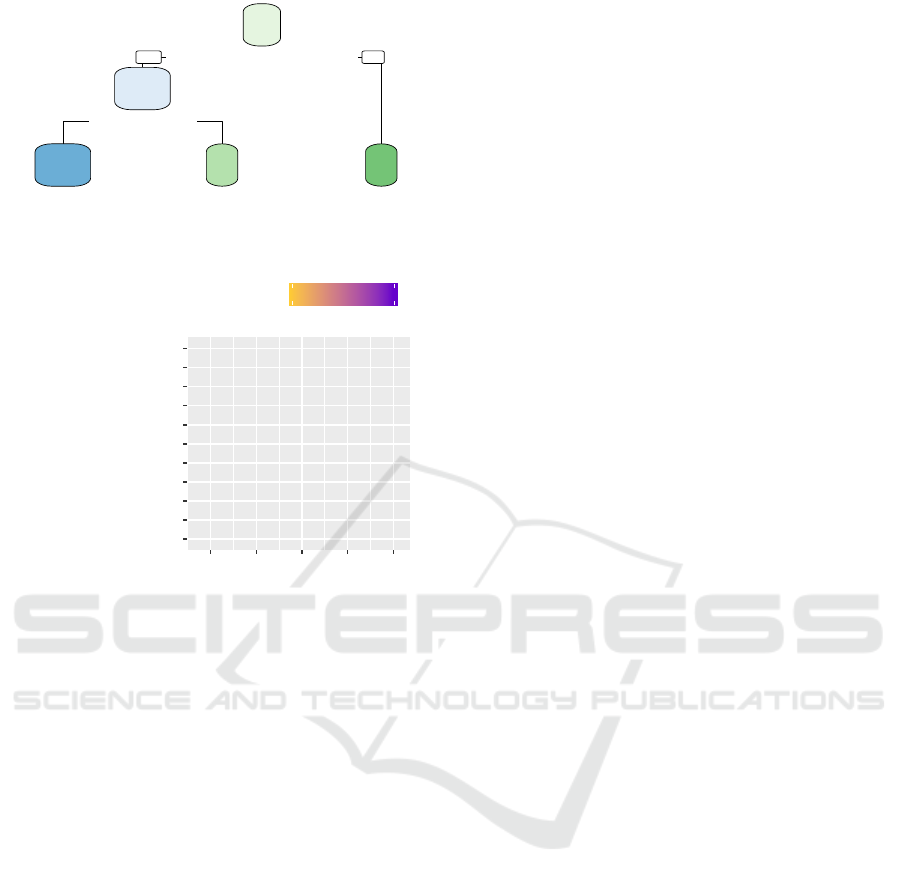
rh_parahippocampal_volume < 0.15

Left.Putamen < 0.28

MCI

0.57

100%

AD

0.38

58%

AD

0.20

39%

MCI

0.75

19%

MCI

0.83

42%

yes

no

Figure 8: CART trained with AIBL and FS1 for MCI vs.

AD. Features are centered and scaled. Nodes: (most fre-

quent class; MCI class probability; coverage).

●

APOE4.0

lh_cuneus_volume

Left.Pallidum

Left.Amygdala

X4th.Ventricle

rh_inferiortemporal_volume

Left.Hippocampus

AGE

Left.Putamen

rh_parahippocampal_volume

lh_precentral_volume

−0.10 −0.05 0.00 0.05 0.10

Shapley value

Feature

Low High

Feature value

Figure 9: SHAP summary plot for the FS1 AIBL XGBoost

model trained for MCI (0) vs. AD (1). APOE4.0 indicates

if a subject had no ApoEε4 alleles. A value of 1 (purple)

expresses a true expression, and 0 (yellow) a false.

applied for the FS1 CARTs trained for the MCI vs.

AD ADNI dataset and the CN vs. MCI AIBL dataset.

The CART trained with FS1 of the AIBL dataset

for MCI vs. AD classiﬁcation is depicted in Figure 8.

All decision values were centered and scaled in this

ﬁgure. For each node, the most frequent class, the

MCI class probability and the coverage in the train-

ing dataset were given. The model was exclusively

based on the volume of the right parahippocampal

gyrus and the left putamen. For both features, subjects

with high volumes were classiﬁed as MCI and sub-

jects with small volumes as AD, which is biologically

plausible but seems to be incomplete, as was noted by

the poor classiﬁcation accuracies of 57.14 % for the

ADNI and 55.77 % for the AIBL test dataset. The RF

and XGBoost black-box models outperformed this

model. The XGBoost model trained on the same

dataset achieved a result of 68.91 % for the ADNI and

70.59 % for the AIBL test dataset. Figure 9 depicts

the SHAP summary plot of this model, which showed

more complex interactions. The most important fea-

ture was the volume of the left precentral gyrus and

high feature values were associated with AD, which

was not biologically plausible. The same applied to

the volume of the left cuneus. All the other detected

associations agreed with the AD neurodegeneration.

Both features included in the CART were present in

the top ten features of the XGBoost model.

Table 6 shows smaller differences between the

CARTs and the black-box models. For example, all

models trained on the CN vs. MCI ADNI dataset re-

ceived the same results of 99.82 % ± 0.41 % during

the CV, 98.91 % for the ADNI and 92.66 % for the

AIBL test dataset. The SHAP summary plot of the

XGBoost model is visualized in Figure 4. This model

was only based on the CDR score. The respective

CART model also used only the CDR score. Since

both models achieved the same classiﬁcation accura-

cies, there was no need to use a complex black-box

model. In conclusion, using black-box models was

more worthwhile for FS1 than for FS2 and sMCI vs.

pMCI classiﬁcation than the BL diagnoses.

5 CONCLUSIONS AND FUTURE

WORK

In this work, several RF, XGBoost and CART mod-

els were trained to classify different AD stages on the

ADNI or AIBL dataset. The models were validated,

using CV and the independent test datasets of both

cohorts. SHAP summary plots were used to visualize

and interpret those models. The experimental results

showed improved accuracies for black-box models

over CARTs. This observation was more clear for the

MCI conversion prediction and for BL diagnoses with

FS1. Simple CARTs were sufﬁcient to classify BL

diagnoses with FS2. One reason for this observation

is that the diagnoses of both cohorts were based on

the cognitive test scores and a neurological examina-

tion (Petersen et al., 2010; Ellis et al., 2009). Conse-

quently, models which included cognitive test scores

achieved better results for the BL classiﬁcation than

models which excluded those features. SHAP sum-

mary plots helped to understand the black-box mod-

els and enabled comparisons between the ADNI and

the AIBL datasets. Those comparisons showed strong

portability for models trained with FS2. Thus, the di-

agnoses and the cognitive test results were similar in

both datasets. Portability of the models between the

ADNI and the AIBL dataset for the CN vs. AD and

sMCI vs. pMCI classiﬁcation with FS1 was also ob-

served. However, no portability between the models

trained for the classiﬁcation of MCI vs. AD and CN

vs. MCI with FS1 was observed. This pointed to rele-

vant differences in the preprocessing or the recording

protocol of the MRI scans in the two studies. Thus,

future experiments should use raw ADNI scans.

HEALTHINF 2021 - 14th International Conference on Health Informatics

96

In future, every article, which uses black-box

models to investigate AD, should also include an in-

terpretation method to explain the model and prove

the biological plausibility. Shapley values provide

suitable model explanations but are not sufﬁcient

to guarantee their biological relevance (Slack et al.,

2020). State-of-the-art methods to measure feature

importance like the RF or the XGBoost feature im-

portance provide a single value per feature. Shap-

ley values, however, enabled to observe complex re-

lationships between feature values and their prognos-

tic relevance, since one Shapley value was calculated

per feature and observation. In these experiments,

the most associations between the feature values and

the predictions were biologically plausible. Individ-

ual predictions, which are important in clinical prac-

tice, can be interpreted using SHAP force plots.

The experiments presented in this paper could be

expanded by including more cohorts like the Open

Access Series of Imaging Studies (OASIS) (Marcus

et al., 2010), a subset of the National Alzheimer’s

Coordinating Center (NACC) (Beekley et al., 2004)

cohort or the AD subset of the HNR study. All ex-

periments used ML models based on DTs. Since

the explanatory method is model-agnostic, the results

should be validated with more diverse ML models and

different interpretable ML methods (Molnar, 2019).

ACKNOWLEDGMENT

Data used in preparation of this article were ob-

tained from the Alzheimer’s Disease Neuroimag-

ing Initiative (ADNI) and the Australian Imaging,

Biomarker & Lifestyle Flagship Study of Ageing

(AIBL) database. We thank the patients and ADNI

and AIBL for availability of the data.

The work of Louise Bloch was partially funded by

a PhD grant from University of Applied Sciences and

Arts Dortmund, Germany.

REFERENCES

Alzheimer’s Association (2020). 2020 Alzheimer’s Dis-

ease facts and ﬁgures. Alzheimer’s & Dementia,

16(3):391–460.

Bartz-Beielstein, T., Lasarczyk, C. W. G., and Preuss, M.

(2005). Sequential parameter optimization. In Pro-

ceesings of the IEEE Congress on Evolutionary Com-

putation, volume 1, pages 773–780.

Beekley, D. L., Ramos, E. M., van Belle, G., Deitrich,

W., Clark, A. D., Jacka, M. E., and Kukull, W. A.

(2004). The National Alzheimer’s Coordinating

Center (NACC) database: An Alzheimer Disease

database. Alzheimer Disease & Associated Disorders,

18(4):270–277.

Bloch, L. and Friedrich, C. M. (2019). Classiﬁcation

of Alzheimer’s Disease using volumetric features of

multiple MRI scans. In Proceedings of the 41st An-

nual International Conference of the IEEE Engineer-

ing in Medicine and Biology Society (EMBC), pages

2396–2401.

Breiman, L. (2001). Random Forests. Machine Learning,

45(1):5–32.

Breiman, L., Friedman, J., Stone, C. J., and Olshen, R. A.

(1984). Classiﬁcation and regression trees. CRC

press, New York, United States, 1st edition.

Chawla, N. V., Bowyer, K. W., Hall, L. O., and Kegelmeyer,

W. P. (2002). SMOTE: Synthetic Minority Over-

sampling Technique. Journal of Artiﬁcial Intelligence

Research, 16(1):321–357.

Chen, T. and Guestrin, C. (2016). XGBoost: A Scalable

Tree Boosting System. In Proceedings of the 22nd

ACM SIGKDD International Conference on Knowl-

edge Discovery and Data Mining, pages 785–794,

New York, United States. ACM.

Chen, T., He, T., Benesty, M., Khotilovich, V., Tang,

Y., Cho, H., Chen, K., Mitchell, R., Cano, I.,

Zhou, T., Li, M., Xie, J., Lin, M., Geng, Y., and

Li, Y. (2019). xgboost: Extreme Gradient Boost-

ing. Manual of R package v0.82.1 https://CRAN.R-

project.org/package=xgboost, Last accessed: 2020-

09-12.

Cortes, C. and Vapnik, V. (1995). Support-vector networks.

Machine Learning, 20(3):273–297.

Das, D., Ito, J., Kadowaki, T., and Tsuda, K. (2019). An

interpretable machine learning model for diagnosis of

Alzheimer’s Disease. PeerJ, 7:e6543.

Desikan, R. S., S

´

egonne, F., Fischl, B., Quinn, B. T., Dick-

erson, B. C., Blacker, D., Buckner, R. L., Dale, A. M.,

Maguire, R. P., Hyman, B. T., Albert, M. S., and Kil-

liany, R. J. (2006). An automated labeling system

for subdividing the human cerebral cortex on MRI

scans into gyral based regions of interest. NeuroIm-

age, 31(3):968–980.

DeTure, M. and Dickson, D. (2019). The neuropathologi-

cal diagnosis of Alzheimer’s Disease. Molecular Neu-

rodegeneration, 14:32.

Dlugaj, M., Weimar, C., Wege, N., Verde, P., Gerwig, M.,

Dragano, N., Moebus, S., J

¨

ockel, K.-H., Erbel, R., and

Siegrist, J. (2010). Prevalence of Mild Cognitive Im-

pairment and its subtypes in the Heinz Nixdorf Recall

Study cohort. Dementia and Geriatric Cognitive Dis-

orders, 30(4):362–373.

Efron, B. and Tibshirani, R. (1986). Bootstrap methods

for standard errors, conﬁdence intervals, and other

measures of statistical accuracy. Statistical Science,

1(1):54–75.

Ellis, K. A., Bush, A. I., Darby, D., De Fazio, D., Fos-

ter, J., Hudson, P., Lautenschlager, N. T., Lenzo, N.,

Martins, R. N., Maruff, P., Masters, C., Milner, A.,

Pike, K., Rowe, C., Savage, G., Szoeke, C., Tad-

dei, K., Villemagne, V., Woodward, M., Ames, D.,

and AIBL Research Group (2009). The Australian

Developing a Machine Learning Workﬂow to Explain Black-box Models for Alzheimer’s Disease Classiﬁcation

97

Imaging, Biomarkers and Lifestyle (AIBL) study of

aging: Methodology and baseline characteristics of

1112 individuals recruited for a longitudinal study of

Alzheimer’s Disease. International Psychogeriatrics,

21(4):672–687.

Fischl, B. (2012). FreeSurfer. NeuroImage, 62(2):774–781.

Fischl, B., Salat, D. H., Busa, E., Albert, M., Dieterich,

M., Haselgrove, C., van der Kouwe, A., Killiany, R.,

Kennedy, D., Klaveness, S., Montillo, A., Makris, N.,

Rosen, B., and Dale, A. M. (2002). Whole brain

segmentation: Automated labeling of neuroanatomi-

cal structures in the human brain. Neuron, 33(3):341–

355.

Friedman, J. H. (2001). Greedy function approximation:

A gradient boosting machine. Annals of Statistics,

29(5):1189–1232.

Goodfellow, I., Pouget-Abadie, J., Mirza, M., Xu, B.,

Warde-Farley, D., Ozair, S., Courville, A., and Ben-

gio, Y. (2014). Generative adversarial nets. In

Advances in neural information processing systems,

pages 2672–2680.

Grassi, M., Rouleaux, N., Caldirola, D., Loewenstein,

D., Schruers, K., Perna, G., Dumontier, M., and

Alzheimer’s Disease Neuroimaging Initiative (2019).

A novel ensemble-based Machine Learning algo-

rithm to predict the conversion from Mild Cogni-

tive Impairment to Alzheimer’s Disease using socio-

demographic characteristics, clinical information, and

neuropsychological measures. Frontiers in Neurology,

10:756.

Greenwell, B. (2020). fastshap: Fast Approximate Shapley

Values. Manual of R package v0.0.5 https://CRAN.R-

project.org/package=fastshap, Last accessed: 2020-

09-12.

Hammond, T. C., Xing, X., Wang, C., Ma, D., Nho, K.,

Crane, P. K., Elahi, F., Ziegler, D. A., Liang, G.,

Cheng, Q., Yanckello, L. M., Jacobs, N., and Lin, A.-

L. (2020). β-amyloid and tau drive early Alzheimer’s

Disease decline while glucose hypometabolism drives

late decline. Communications Biology, 3(1).

Hochreiter, S. and Schmidhuber, J. (1997). Long Short-

Term Memory. Neural computation, 9(8):1735–1780.

Jack, C. R., Barnes, J., Bernstein, M. A., Borowski, B. J.,

Brewer, J., Clegg, S., Dale, A. M., Carmichael, O.,

Ching, C., DeCarli, C., Desikan, R. S., Fennema-

Notestine, C., Fjell, A. M., Fletcher, E., Fox, N. C.,

Gunter, J., Gutman, B. A., Holland, D., Hua, X., Insel,

P., Kantarci, K., Killiany, R. J., Krueger, G., Leung,

K. K., Mackin, S., Maillard, P., Molone, I., Mattsson,

N., McEvoy, L., Modat, M., Mueller, S., Nosheny, R.,

Ourselin, S., Schuff, N., Senjem, M. L., Simonson,

A., Thompson, P. M., Rettmann, D., Vemuri, P., Wal-

hovd, K., Zhao, Y., Zuk, S., and Weiner, M. (2015).

Magnetic Resonance Imaging in ADNI. Alzheimer’s

& dementia, 11(7):740–756.

Kuhn, M. (2019). caret: Classiﬁcation and Regres-

sion Training. Manual of R package v6.0-82

https://CRAN.R-project.org/package=caret, Last ac-

cessed: 2020-09-12.

LeCun, Y., Bengio, Y., and Hinton, G. (2015). Deep learn-

ing. Nature, 521(7553):436–444.

Li, M., Reisman, J., Morris-Eppolito, B., Qian, S. X.,

Kazis, L. E., Wolozin, B., Goldstein, L. E., and Xia,

W. (2020). Beneﬁcial association of angiotensin-

converting enzyme inhibitors and statins on the occur-

rence of possible Alzheimer’s Disease after traumatic

brain injury. Alzheimer’s Research & Therapy, 12(1).

Liaw, A. and Wiener, M. (2002). Classiﬁcation and Regres-

sion by randomForest. R News, 2(3):18–22.

Lloret, A., Esteve, D., Lloret, M.-A., Cervera-Ferri, A.,

Lopez, B., Nepomuceno, M., and Monllor, P. (2019).

When does Alzheimer’s Disease really start? The role

of biomarkers. International Journal of Molecular

Sciences, 20(22):5536.

Lundberg, S. M., Erion, G. G., and Lee, S. (2018).

Consistent individualized feature attribution for

tree ensembles. Computing Research Repository.

http://arxiv.org/abs/1802.03888, Last accessed: 2020-

09-13.

Lundberg, S. M. and Lee, S.-I. (2017). A uniﬁed ap-

proach to interpreting model predictions. In Guyon,

I., Luxburg, U. V., Bengio, S., Wallach, H., Fer-

gus, R., Vishwanathan, S., and Garnett, R., editors,

Advances in Neural Information Processing Systems,

volume 30, pages 4765–4774. Curran Associates, Inc.

Marcus, D. S., Fotenos, A. F., Csernansky, J. G., Morris,

J. C., and Buckner, R. L. (2010). Open Access Series

of Imaging Studies: Longitudinal MRI data in nonde-

mented and demented older adults. Journal of Cogni-

tive Neuroscience, 22(12):2677–2684.

McKay, M. D., Beckman, R. J., and Conover, W. J. (1979).

A Comparison of three methods for selecting values of

input variables in the analysis of output from a com-

puter code. Technometrics, 21(2):239–245.

Mo

ˇ

ckus, J. (1975). On bayesian methods for seeking the

extremum. In Proceedings of the Optimization Tech-

niques IFIP Technical Conference, pages 400–404.

Springer.

Mofrad, R. B., Schoonenboom, N. S., Tijms, B. M., Schel-

tens, P., Visser, P. J., Flier, W. M., and Teunissen, C. E.

(2018). Decision tree supports the interpretation of

CSF biomarkers in Alzheimer’s Disease. Alzheimer’s

& Dementia: Diagnosis, Assessment & Disease Mon-

itoring, 11(1):1–9.

Molnar, C. (2019). Interpretable Machine Learning:

A guide for making black box models explain-

able. https://christophm.github.io/interpretable-ml-

book/, Last accessed: 2020-08-30.

Patterson, C. (2018). World Alzheimer report

2018 - The state of the art of dementia re-

search: New frontiers. Alzheimer’s Dis-

ease International, London, Great Britain.

https://www.alz.co.uk/research/WorldAlzheimerRepo

rt2018.pdf, Last accessed: 2020-08-26.

Pelka, O., Friedrich, C. M., Nensa, F., M

¨

onninghoff, C.,

Bloch, L., J

¨

ockel, K.-H., Schramm, S., Sanchez Hoff-

mann, S., Winkler, A., Weimar, C., Jokisch, M., and

for the Alzheimer’s Disease Neuroimaging Initiative

(2020). Sociodemographic data and APOE- 4 aug-

mentation for MRI-based detection of amnestic Mild

Cognitive Impairment using deep learning systems.

PLOS ONE, 15(9):1–24.

HEALTHINF 2021 - 14th International Conference on Health Informatics

98

Petersen, R. C., Aisen, P. S., Beckett, L. A., Donohue,

M. C., Gamst, A. C., Harvey, D. J., Jack, C. R., Jagust,

W. J., Shaw, L. M., Toga, A. W., Trojanowski, J. Q.,

and Weiner, M. W. (2010). Alzheimer’s Disease Neu-

roimaging Initiative (ADNI). Neurology, 74(3):201–

209.

R Core Team (2019). R: A language and environment

for statistical computing. R Foundation for Statis-

tical Computing, Vienna, Austria. Manual v3.5.3

https://www.R-project.org/, Last accessed: 2020-09-

12.

Refaeilzadeh, P., Tang, L., and Liu, H. (2009). Cross-

Validation. In Liu, L. and

¨

Ozsu, M. T., editors,

Encyclopedia of Database Systems, pages 532–538,

Boston, United States. Springer.

Rieke, J., Eitel, F., Weygandt, M., Haynes, J.-D., and Rit-

ter, K. (2018). Visualizing Convolutional Networks

for MRI-based diagnosis of Alzheimer’s Disease. In

Stoyanov, D., Taylor, Z., Kia, S. M., Oguz, I., Reyes,

M., Martel, A., Maier-Hein, L., Marquand, A. F.,

Duchesnay, E., L

¨

ofstedt, T., Landman, B., Cardoso,

M. J., Silva, C. A., Pereira, S., and Meier, R., editors,

Understanding and interpreting Machine Learning in

medical image computing applications, pages 24–31.

Springer International Publishing.

Rumelhart, D. E., Hinton, G. E., and Williams, R. J. (1986).

Learning representations by back-propagating errors.

Nature, 323(6088):533–536.

Samper-Gonz

´

alez, J., Burgos, N., Bottani, S., Fontanella,

S., Lu, P., Marcoux, A., Routier, A., Guillon, J., Bacci,

M., Wen, J., Bertrand, A., Bertin, H., Habert, M.-O.,

Durrleman, S., Evgeniou, T., and Colliot, O. (2018).

Reproducible evaluation of classiﬁcation methods in

Alzheimer’s Disease: Framework and application to

MRI and PET data. NeuroImage, 183:504–521.

Schmermund, A., M

¨

ohlenkamp, S., Stang, A., Gr

¨

onemeyer,

D., Seibel, R., Hirche, H., Mann, K., Siffert, W.,

Lauterbach, K., Siegrist, J., J

¨

ockel, K.-H., and Erbel,

R. (2002). Assessment of clinically silent atheroscle-

rotic disease and established and novel risk factors for

predicting myocardial infarction and cardiac death in

healthy middle-aged subjects: Rationale and design of

the Heinz Nixdorf RECALL study. American Heart

Journal, 144(2):212–218.

Selvaraju, R. R., Cogswell, M., Das, A., Vedantam, R.,

Parikh, D., and Batra, D. (2017). Grad-CAM: Vi-

sual Explanations from Deep Networks via Gradient-

Based Localization. In Proceedings of the IEEE In-

ternational Conference on Computer Vision (ICCV),

pages 618–626.

Shapley, L. S. (1953). A Value for n-Person Games. In

Kuhn, H. W. and Tucker, A. W., editors, Contributions

to the Theory of Games (AM-28), volume 2, pages

307–318. Princeton University Press.

Simonyan, K., Vedaldi, A., and Zisserman, A. (2014). Deep

inside convolutional networks: Visualising image

classiﬁcation models and saliency maps. Computing

Research Repository. http://arxiv.org/abs/1312.6034,

Last accessed: 2020-08-30.

Slack, D., Hilgard, S., Jia, E., Singh, S., and Lakkaraju, H.

(2020). Fooling LIME and SHAP adversarial attacks

on post hoc explanation methods. In Proceedings of

the AAAI/ACM Conference on AI, Ethics, and Society.

ACM.

Springenberg, J., Dosovitskiy, A., Brox, T., and Ried-

miller, M. (2015). Striving for simplicity: The

all Convolutional Net. In Proceedings of the In-

ternational Conference on Learning Representations

(ICLR) (workshop track). http://lmb.informatik.uni-

freiburg.de/Publications/2015/DB15a, Last accessed:

2020-08-30.

ˇ

Strumbelj, E. and Kononenko, I. (2013). Explaining pre-

diction models and individual predictions with feature

contributions. Knowledge and Information Systems,

41(3):647–665.

Therneau, T. and Atkinson, B. (2018). rpart: Re-

cursive Partitioning and Regression Trees.

Manual of R package v4.1-13 https://CRAN.R-

project.org/package=rpart, Last accessed: 2020-09-

12.

Wang, X., Shen, D., and Huang, H. (2019). Interpretable

deep temporal structure learning model for early de-

tection of Alzheimer’s Disease. bioRxiv.

Wen, J., Thibeau-Sutre, E., Diaz-Melo, M., Samper-

Gonz

´

alez, J., Routier, A., Bottani, S., Dormont, D.,

Durrleman, S., Burgos, N., and Colliot, O. (2020).

Convolutional Neural Networks for classiﬁcation of

Alzheimer’s Disease: Overview and reproducible

evaluation. Medical Image Analysis, 63:101694.

Westman, E., Aguilar, C., Muehlboeck, J.-S., and Simmons,

A. (2012). Regional Magnetic Resonance Imaging

measures for multivariate analysis in Alzheimer’s Dis-

ease and Mild Cognitive Impairment. Brain Topogra-

phy, 26(1):9–23.

Yan, Y. (2016). rBayesianOptimization: Bayesian

Optimization of Hyperparameters. Man-

ual of R package v1.1.0 https://CRAN.R-

project.org/package=rBayesianOptimization, Last

accessed: 2020-09-12.

Yang, C., Rangarajan, A., and Ranka, S. (2018). Vi-

sual explanations from deep 3D Convolutional

Neural Networks for Alzheimer’s Disease clas-

siﬁcation. Computing Research Repository.

http://arxiv.org/abs/1803.02544, Last accessed:

2020-08-30.

Zeiler, M. D. and Fergus, R. (2014). Visualizing and under-

standing Convolutional Networks. In Fleet, D., Pajdla,

T., Schiele, B., and Tuytelaars, T., editors, Proceed-

ings of the 13th European Conference on Computer

Vision (ECCV), pages 818–833. Springer International

Publishing.

Developing a Machine Learning Workﬂow to Explain Black-box Models for Alzheimer’s Disease Classiﬁcation

99