Synthesis of Non-homogeneous Textures by Laplacian Pyramid

Coefﬁcient Mixing

Das Moitry and David Mould

School of Computer Science, Carleton University, Ottawa, Canada

Keywords:

Texture Synthesis, Texture Blending, Laplacian Pyramids, Image Processing.

Abstract:

We present an example-based method for generating non-homogeneous stochastic textures, where the output

texture contains elements from two input exemplars. We provide user control over the blend through a blend

factor that speciﬁes the degree to which one texture or the other should be favored; the blend factor can vary

spatially. Uniquely, we add spatial coherence to the output texture by performing a joint oversegmentation

of the two texture inputs, then applying a ﬁxed blend factor within each segment. Our method works with

the Laplacian pyramid representation of the textures. We combine the pyramid coefﬁcients using a weighted

smooth maximum, ensuring that locally prominent features are preserved through the blending process. Our

method is effective for stochastic textures and successfully blends the structures of the two inputs.

1 INTRODUCTION

Texture is a key element in synthetic and modiﬁed

images, used to add detail and visual interest to a

rendered scene. Example-based synthesis algorithms,

including modern machine-learning based methods,

have been quite successful for stationary textures.

However, there has been comparatively less success

at non-homogeneous textures, where the texture’s ap-

pearance varies over the image plane. In this paper,

we describe a method for generating blends between

two input textures, where the degree to which one tex-

ture is favored over the other changes with spatial lo-

cation within the image. Our method is best adapted

to stochastic, unstructured textures.

Our method can be used directly for texture syn-

thesis, blending between two input exemplars, with

the output texture being applied to geometry in a

conventional rendering pipeline. However, in many

cases, it is not a priori obvious what texture might

be intermediate between two textures. Thus, another

possible application of our method is in texture de-

sign, allowing a texture artist to explore a space of

textures generated by mixing different exemplars.

Our method takes as input exemplars of stochastic

texture. For generating a large output of required size,

we use the method of Heitz and Neyret (Heitz and

Neyret, 2018) which employs histogram-preserving

blending. We can also use textures as input directly,

bypassing the histogram-preserving blending stage.

Once we have two textures of matching size, we

blend them within their Laplacian pyramid represen-

tations. Enforcing the same size on the two inputs

ensures that there is a one-to-one correspondence be-

tween the coefﬁcients in the two Laplacian pyramids.

We mix the pyramid coefﬁcients using a weighted

smooth maximum; the smooth maximum ensures that

strong features, manifesting as large coefﬁcient mag-

nitudes, are preserved. By weighting the inputs ac-

cording to a user-controllable local blend factor, we

can control the degree of blending spatially.

As an optional ﬁnal step, we can further increase

the heterogeneity of the texture blend by preserving

larger texture chunks. We conduct an oversegmen-

tation of the image plane using Simple Linear Itera-

tive Clustering (SLIC), and then for each segment, we

merge the inputs with a blend factor weighted towards

one or the other texture. The result has distinct frag-

ments of texture, as opposed to the more continuous

blend we would otherwise see.

This paper presents a framework for merging

stochastic textures with local control over the degree

to which one texture or the other is more promi-

nent. The outputs have features from both inputs, with

strong features being preserved in a perceptually ap-

pealing way. Supporting this work, this paper makes

the following technical contributions:

• Structural texture blending of stochastic textures,

using the smooth maximum to mix coefﬁcients of

the Laplacian pyramid.

Moitry, D. and Mould, D.

Synthesis of Non-homogeneous Textures by Laplacian Pyramid Coefﬁcient Mixing.

DOI: 10.5220/0010204601610168

In Proceedings of the 16th International Joint Conference on Computer Vision, Imaging and Computer Graphics Theory and Applications (VISIGRAPP 2021) - Volume 1: GRAPP, pages

161-168

ISBN: 978-989-758-488-6

161

• Adding texture heterogeneity through a joint

SLIC segmentation of both input textures.

• Use of a weighted smooth maximum for control-

lable and spatially varying texture mixing.

• An overall framework for synthesizing non-

homogeneous stochastic textures from exemplars.

Given exemplars, we use histogram-preserving

blending to generate full-size textures, then blend

them in a Laplacian pyramid representation.

In the remainder of the paper, we ﬁrst discuss

background and related work, then move on to de-

scribing our algorithm in detail. We show results and

discuss some speciﬁc features of our output in Sec-

tion 4. We close in Section 5 and give some sugges-

tions for future work.

2 BACKGROUND

Early texture synthesis methods were based on ma-

nipulating structured noise, such as Perlin noise or

Worley noise. Such methods were ad hoc and dif-

ﬁcult to generalize. Later example-based synthesis

methods were considered easier to control: example-

based texture synthesis aims at creating new tex-

ture images from an input sample, with both pixel-

based (Efros and Leung, 1999; Ashikhmin, 2001)

and patch-based (Efros and Freeman, 2001) methods

proposed. An early effort at example-based synthe-

sis by Heeger and Bergen made use of image pyra-

mids (Heeger and Bergen, 1995). More recently,

methods based on machine learning have received

considerable attention (Gatys et al., 2015; Sendik and

Cohen-Or, 2017).

Early work on non-homogeneous textures was

conducted by Zhang et al. (Zhang et al., 2003), who

blended binary texton maps from two inputs to create

a progression from one texture to the other. More re-

cently, both Zhou et al. (Zhou et al., 2017) and Lock-

erman et al. (Lockerman et al., 2016) gave methods

to construct a label map from a non-homogeneous ex-

emplar. Zhou et al. (Zhou et al., 2018) used genera-

tive adversarial networks to synthesize non-stationary

textures from a guidance map.

Heitz and Neyret proposed texture synthesis

through histogram-preserving blending (Heitz and

Neyret, 2018). We discuss this method in more detail

as it forms one stage of our own synthesis process.

Their method works as follows. They take in an

exemplar of a stochastic texture. They apply a his-

togram transformation so that the resulting texture’s

color distribution is a Gaussian. They then generate

a new texture sample by blending patches from the

Gaussianized exemplar; the key insight is that since

the patches have Gaussian histograms, the blending

can incorporate a function that preserves the same

Gaussian histogram in the output. Once the blended

texture is computed, the inverse histogram transfor-

mation can be applied to restore the original texture

distribution.

Their method then restores the original color

distribution, computing an optimal transport match-

ing (Bonneel et al., 2016) between the original tex-

ture colors and the Gaussianized colors. The overall

method is fast and effective, creating new texture that

resembles the exemplar. The method does not work

on structured textures, a drawback that our method

shares due to (a) our use of HPB in an early stage, and

(b) our use of Laplacian pyramid coefﬁcient mixing,

ill-suited to merging dissimilar structured images.

We will make use of the smooth maximum func-

tion (Cook, 2010). The smooth maximum of two vari-

ables x and y is given by

g(x,y) = log(exp(x) + exp(y)). (1)

When one of the inputs is much larger than the other,

the smooth maximum converges to the regular maxi-

mum. When the inputs are closer to equal, however,

the smooth maximum produces an output larger than

either. The function is designed to avoid any sudden

discontinuity in behaviour as the values of the inputs

change. We use a variant of the smooth maximum for

mixing coefﬁcients in the Laplacian pyramid repre-

sentation of the textures.

3 ALGORITHM

We present an algorithm for blending two input tex-

tures. The process follows these steps:

• We establish our inputs, often synthesized from

exemplars using histogram-preserving blending.

• We compute the Laplacian pyramid of each tex-

ture. We then compute a merged pyramid by mix-

ing the corresponding coefﬁcients at every level

in the input pyramids, using a weighted smooth

maximum to ﬁnd the output coefﬁcient. The out-

put pyramid is then collapsed to create an output

texture.

• Optionally, we oversegment the output plane, then

blend with a ﬁxed blend factor within each seg-

ment. This step creates macroscopic regions that

strongly favor one texture or the other, increasing

the texture heterogeneity.

• The Laplacian pyramid is done in greyscale only.

We determine a color for each pixel, choosing one

GRAPP 2021 - 16th International Conference on Computer Graphics Theory and Applications

162

input color or the other, based on which texture’s

Laplacian coefﬁcients more inﬂuenced this pixel’s

intensity.

In the following subsections, we describe each of

these steps in greater detail.

3.1 Histogram Preserving Blending

We take in two texture samples, A and B. We then

use histogram-preserving blending (HPB) (Heitz and

Neyret, 2018) to generate textures A

and B

each of

the desired output size. We will then blend A

and

using the Laplacian pyramid. The use of HPB al-

lows us to generate many distinct textures from a sin-

gle pair of examplars.

3.2 Blending Coefﬁcients

We compute the Laplacian pyramids L

and L

inputs A

and B

respectively. We aim to compute an

output pyramid L

, blending the coefﬁcients of L

and L

using a weighted smooth maximum function.

The weights are controlled by a blend factor t and by

an estimate of the texture activity level. The smooth

maximum prioritizes the larger coefﬁcient, so weight-

ing by texture activity presents a higher-contrast tex-

ture with larger-magnitude coefﬁcients from over-

whelming the other texture.

The blend factor 0 ≤ t ≤ 1 indicates the desired

proportions of the two inputs. It can be be a constant

over the image, or a ﬁeld over the image plane. We

typically show results with t as a function of horizon-

tal distance: t = 0 at the left-hand image edge, rising

linearly to t = 1 at the right edge.

We estimate the strength of each texture from the

root mean squared (RMS) average of the coefﬁcients

at each pyramid level. We then average the RMS

scores at each level, weighted by the blend factor;

this average inﬂuences the weighted smooth maxi-

mum used in the coefﬁcient mixing. More formally,

the output coefﬁcients are computed using a weighted

smooth maximum. For inputs x and y, with weights

p and q respectively, we formulated the weighted

smooth maximum as follows:

SM(x,y, p, q) =

√

pq + ε



ln(exp(px) + exp(qy)−1)



(2)

When p > q, the result will tend more towards x;

when p < q, the result tends towards y. We subtract

one from the sum of the exponentiated inputs to re-

move upward bias: when both inputs are zero then

the output will also be zero. The small value ε guards

against division by zero.

Given Equation 2, we need to decide on suitable

weights. It would be natural to simply use the blend

factor as the weight: texture A would have weight

(1 −t) and texture B would have weight t. However,

suppose one texture had greater variability than the

other, hence generally larger coefﬁcients. This texture

would dominate and its features would show through

the relatively lower-amplitude texture, even when the

blend factor indicated otherwise.

We normalize the coefﬁcients of each pyramid

level according to their root mean square. Let g

and

be the RMS of level l’s coefﬁcients for A

and B

respectively. The normalization factor a is then com-

puted as follows:

= (1 −t) ·g

+t ·h

. (3)

The value a

is the average of the two input RMS val-

ues, weighted by the blend factor t. Consider a to be a

target amplitude, governing the amplitude of the out-

put texture. We then assign coefﬁcient weights based

on the ratio of a to each texture’s RMS, as follows:

= a

(4)

= a

(5)

We calculate ﬁnal weights p

and q

in Eqn. 6 and

Eqn. 7. Notice that t is in effect included twice: once

to compute the local normalization factor in Eqn.3

and once to blend between the normalized coefﬁ-

cients. The weights p

and q

will be used to do our

ﬁnal coefﬁcient mixing.

= p

·(1 −t) (6)

= q

·t (7)

Finally, we compute each output coefﬁcient

(x,y) at level l as follows. Each level of the resul-

tant Laplacian pyramid L

will be constructed with

the resultant merged coefﬁcients.

(x,y) = Ψ ×SM





(x,y)



(x,y)



, p



(8)

In the preceding, the variable Ψ ∈ {−1,1} is the

sign of the coefﬁcient which has the larger absolute

value after weighting. Combining all the levels of

, we form an output image merging the textures A

and B

. The blended greyscale image exhibits features

of both inputs, distributed depending on the map of

blend factor values t.

An example result is give in Figure 1, show-

ing blending between two textures for different ﬁxed

blend factors. In this example, the blend factor t is

ﬁxed at a single value over the entire image plane.For

small t, the output resembles the ﬁrst input; as t ap-

proaches 1, the output resembles the second input.

Synthesis of Non-homogeneous Textures by Laplacian Pyramid Coefﬁcient Mixing

163

Intermediate values of t show elements from both in-

puts, without the unappealing blurring of features that

is characteristic of alpha blending.

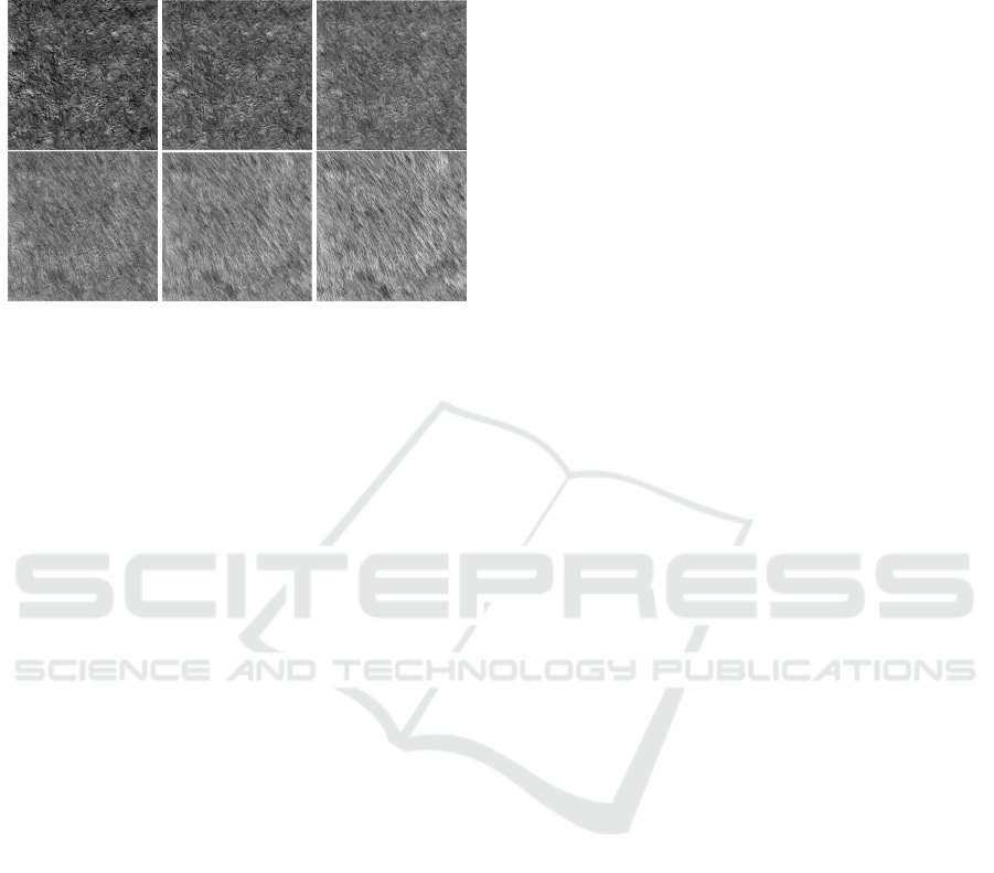
Figure 1: Texture blending with ﬁxed t. Above: t = 0.0,

t = 0.2, t = 0.4. Below: t = 0.6, t = 0.8, t = 1.0.

3.3 Recoloring

Above, we compute the Laplacian coefﬁcients of the

greyscale image. Attempting to merge three sets of

coefﬁcients in a 3D colorspace yields unsatisfactory

results. In this step, we ﬁnalize our texture by adding

color.

Each output pixel is governed by h coefﬁcients,

where h is the height of the Laplacian pyramid. We

compare each coefﬁcient in the output pyramid with

the corresponding coefﬁcients in the pyramids of the

two inputs. We assign a score of +1 if the output co-

efﬁcient is nearer to the ﬁrst input’s coefﬁcient, and

−1 otherwise. For each output pixel, we take the sum

of the scores of the relevant coefﬁcients. This can be

thought of as a voting mechanism: if the ﬁnal score is

positive, the ﬁrst input has greater inﬂuence, and if the

score is negative, the second input has greater inﬂu-

ence. Then, maintaining its intensity, we assign to this

pixel the color of the higher-inﬂuence input. Repeat-

ing over all pixels, we can color the entire output tex-

ture. Note that individual coefﬁcient scores need not

be calculated repeatedly, but can be computed once

and saved in a data structure paralleling the Laplacian

pyramid, with the coloring being implemented as a

specialized form of pyramid collapse.

3.4 Additional Heterogeneity

We close by describing an optional step to increase

output heterogeneity. With the above, we are able to

create gradual blends between textures. However, in-

termediate texture structures may not be desirable; in

many natural examples of mixed textures, there are

distinct regions where one texture type or the other is

dominant. Consider, for example, a stone face with

occasional plant growth, or a pavement partly cov-

ered by snow, or an old car door with peeling paint.

In these cases, there are areas where one texture is

prevalent and areas that favor the other.

Accordingly, we suggest creating a spatial struc-

ture that helps assign values to the local blend factor.

We apply an oversegmentation to the image plane,

and within a given segment, we will favor one tex-

ture or the other. We will still interpolate between our

two inputs; now, the choice of which texture to fa-

vor will be determined by the location of the region,

such that the majority of regions on the left will be

assigned to the ﬁrst input, and the regions on the right

will be predominantly assigned to the second input.

More formally, for a normalized distance t across the

horizontal dimension of the image plane, we assign a

segment the probability 1 −t of favoring the ﬁrst in-

put, and probability t of favoring the second.

The oversegmentation itself is computed taking

into account both inputs. We perform a joint SLIC

segmentation (Achanta et al., 2012) of the two in-

puts: recall that SLIC operates in a distance+color

5D space, and we amend it now to use two color dis-

tances, one for each input, weighted by the local blend

factor. Formally, the SLIC distance is given by

D(x,y) = sqrt((x −x

)

+ (y −y

)

+ (1 −t)||C

(x,y) −C

)||

+t||C

(x,y) −C

)||

for input color textures C

and C

and a region cen-

troid located at x

. The choice of SLIC for the

segmentation ensures approximately equal-sized re-

gions throughout the image plane. Incorporating the

color distance for both input textures allows the re-

gion boundaries to take into account texton shapes.

Figure 3 provides a visual example of the region

boundaries obtained for two sample inputs.

Once the coefﬁcients are blended, we keep only

the blended coefﬁcients within the original SLIC seg-

ment boundary from the bounded square. We discard

the rest since the bounded square was created only for

generating the Laplacian pyramid. The coefﬁcients

that were not discarded form a temporary pyramid

that can be collapsed to produce pixel values within

the segment. Once the pixel values within the seg-

ment have been computed, we discard the temporary

pyramid. This is done for all K of the SLIC segments.

The treatment of the Laplacian coefﬁcients is akin to

that given by Paris et al. (Paris et al., 2011).

Figure 3 shows the region map with SLIC seg-

ments, showing how the input textures will dis-

tributed. The regions shown in blue will be populated

primarily with the ﬁrst input and the white regions

GRAPP 2021 - 16th International Conference on Computer Graphics Theory and Applications

164

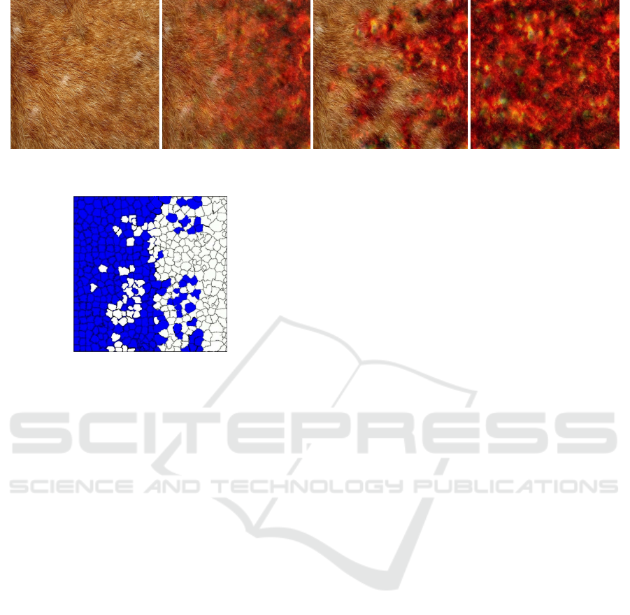
Figure 2: Comparison of results with and without oversegmentation-based heterogeneity. First and last images: input textures.

Centre left: continuous blend. Centre right: blend with oversegmentation controlling blend factor.

Figure 3: Oversegmentation map. Blue regions will be pre-

dominantly one texture, white regions the other.

will be populated with the second.

Through this optional additional step we can add

further heterogeneity to the texture, giving a scattered

and irregular distribution of texture contents from

both inputs throughout the output image. While not

needed in all cases, this simple label map provides an

additional tool for creating a desired effect.

4 RESULTS AND DISCUSSION

Here, we discuss some results. Figure 4 shows re-

sults from our full pipeline, including histogram-

preserving blending. Figure 5 shows results on arbi-

trary inputs, omitting the histogram-preserving blend-

ing step in favor of using the exemplars directly. Fig-

ure 6 shows a result from blending two textures with

a hand-drawn map. Finally, Figure 7 shows a fail-

ure case from applying our technique on highly struc-

tured brick texture. We discuss each of these ﬁgures

in more detail below.

Figure 4 shows several results of structural tex-

ture blending. Consider ﬁrst the topmost blend in

Figure 4. The textures are dissimilar: the rock is

largely isotropic, while the fur exhibits strong direc-

tionality. However, the texture structures merge ef-

fectively, with fur structures giving way to higher-

frequency roughness and vice versa. The reader is

invited to look closely at the blended region near the

lower left of the image, where elements of both tex-

tures integrate particularly harmoniously.

For more similar inputs, the results are even more

convincing. Consider the blend in the second row in

Figure 4, showing a transition between two rock tex-

tures. The small-scale structures ﬂow seamlessly into

one another; at some locations one texture dominates,

and at some locations another, but the continuity be-

tween structures is excellent. The use of smooth max-

imum ensures that a strong feature is not lost unless it

is covered by an even stronger feature. Examples of

good local transitions abound.

The third row shows a blend between two distinc-

tive colors. Here, we did not use oversegmentation;

the blend factor changes linearly from left to right.

The textures merge seamlessly, with features from

each integrating nicely. There is no ghosting as would

have been produced by alpha blending.

The fourth row shows an oversegmentation-based

blend between granite and lava textures with dissim-

ilar structures and similar colors. The result is good

structurally. The color mixing is plausible, partially

due to the compatibility of the inputs.

The ﬁfth row shows a blend between two textures

dissimilar both in structure and in color. The overseg-

mentation produces islands of one color or the other.

Although the colors do not blend neatly here, the re-

sult admits a semantic interpretation of water sinking

into sand. This result shows the limitation of our color

blending process in the oversegmentation context and

points the way towards future work.

Figure 5 shows two results from blending in-

puts directly, without the step of histogram-preserving

blending to create new texture. None of the textures

shown could have been recreated with histogram-

preserving blending. In the top row, we see a mix

of stone and grass textures. The result scatters small

patches of greenery across the grey stone. The tex-

ture suggests a rough surface throughout, occasion-

ally covered but not concealed by a veneer of plant

life. In the bottom row, we see a complex stone face

merge with lichens. Again, the structural preservation

Synthesis of Non-homogeneous Textures by Laplacian Pyramid Coefﬁcient Mixing

165

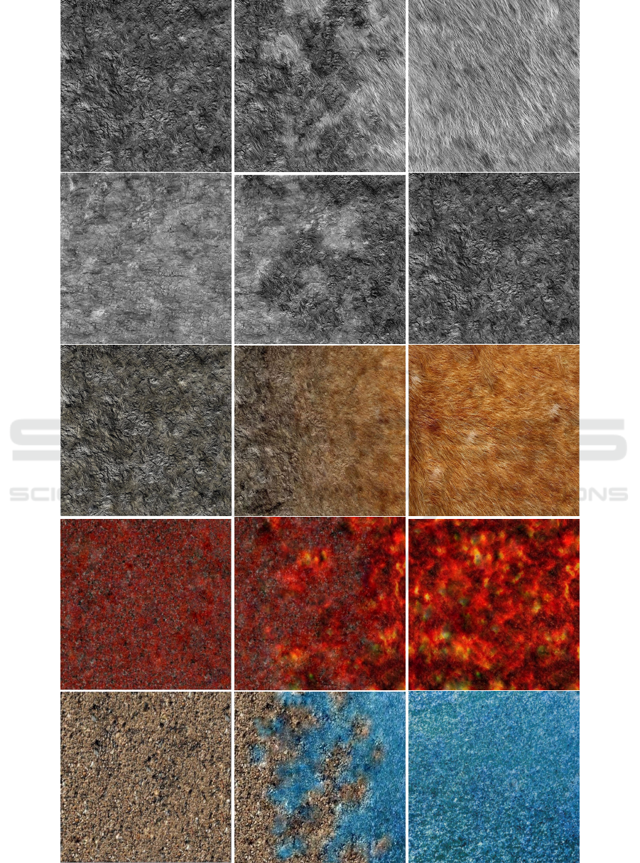
Figure 4: Texture blending results using histogram-preserving blending to generate inputs. Left column: input 1; middle

column: blended output; right column: input 2.

GRAPP 2021 - 16th International Conference on Computer Graphics Theory and Applications

166

Figure 5: Sample results with arbitrary inputs. Left column: input 1; middle column: blended output; right column: input 2.

Figure 6: Controlling the blending factor with a handmade

map. Above: two inputs. Lower left: visualization of map.

Lower left: blended texture.

Figure 7: Failure case on structured inputs. The blended

output exhibits signiﬁcant ghosting artifacts.

is good, with the lichens seeming to conform to the

shapes in the stone. In both examples, we use over-

segmentation, with a blend factor favoring the left in-

put on the left side of the output, and favoring the right

input towards the right.

We typically blended textures with a blend factor

that varied smoothly from left to right. This was done

for consistency and for convenience of interpretation

rather than any technical limitation. Figure 6 shows a

result from blending two textures with a hand-drawn

map of blend factors. Despite the low level of simi-

larity between the input textures, we obtain a merged

texture with structural consistency across the texture

boundary.

In general, our method is effective within the do-

main for which it was intended: blending between

two stochastic textures, with local variation of the

blend factor. However, the features of regular tex-

tures are blended less plausibly. The bricks in Fig-

ure 7 provide an example. Of course, the brick tex-

tures could not have been recreated by histogram-

preserving blending in the ﬁrst place.

Our method has other limitations. Our efforts at

normalizing the texture intensity were only partially

successful: when two textures with radically differ-

ent contrasts are blended, the results are not entirely

satisfactory. Future work will further investigate tex-

Synthesis of Non-homogeneous Textures by Laplacian Pyramid Coefﬁcient Mixing

167

tures with very different levels of intensity variation.

Color restoration could also be improved. Compat-

ible palettes yield convincing results, but dissimilar

palettes are integrated less well. Better color blend-

ing, especially in conjunction with oversegmentation,

is a direction for future work. The sign of the output

coefﬁcient (positive or negative) is decided separately

from the magnitude and is a binary outcome. While

generally effective for static textures, the process has

a discontinuity as the two input values become simi-

lar in magnitude, which could be a problem for future

efforts on dynamic textures.

5 CONCLUSIONS AND FUTURE

WORK

We presented a method for synthesizing textures in-

termediate between two exemplars. The degree of

blending can vary spatially, yielding inhomogeneous

textures if desired. Using the SLIC segments we were

able increase heterogeneity, preserving small coher-

ent regions of each texture.

Our process is applicable only for textures lacking

well-deﬁned structures. It also has difﬁculty preserv-

ing long continuous features. However, for stochastic

textures with small features, our output textures look

realistic and natural. In future work, we would like

to consider additional factors, including local con-

trast and directionality. We would like to extend the

method to work well for more structured textures. We

would also like to use time as a factor in order to cre-

ate dynamic textures.

In this work, we treated all levels of the Laplacian

pyramid the same way. However, it might make sense

to investigate different treatments for different levels.

Depending on the texture, one level or another may

contain more of the structural content, and account-

ing for this in the merging could produce still bet-

ter blends. The example of Doyle and Mould (Doyle

and Mould, 2018) is instructive, albeit not in a texture

blending context.

ACKNOWLEDGEMENTS

This work was supported by the Natural Sciences and

Engineering Research Council of Canada. We thank

members of the Graphics, Imaging, and Games Lab at

Carleton University for many useful discussions dur-

ing the development of this work. Finally, thanks to

the reviewers for helpful comments.

REFERENCES

Achanta, R., Shaji, A., Smith, K., Lucchi, A., Fua, P., and

usstrunk, S. (2012). SLIC superpixels compared to

state-of-the-art superpixel methods. IEEE Transac-

tions on Pattern Analysis and Machine Intelligence,

34(11):2274–2282.

Ashikhmin, M. (2001). Synthesizing natural textures. In

Proceedings of the 2001 Symposium on Interactive 3D

Graphics, I3D ’01, page 217–226, New York, NY,

USA. Association for Computing Machinery.

Bonneel, N., Peyr

e, G., and Cuturi, M. (2016). Wasserstein

barycentric coordinates: Histogram regression using

optimal transport. ACM Trans. Graph., 35(4).

Cook, J. D. (2010). Soft maximum.

Doyle, L. and Mould, D. (2018). Augmenting photographs

with textures using the Laplacian pyramid. The Visual

Computer, pages 1–12.

Efros, A. A. and Freeman, W. T. (2001). Image quilting for

texture synthesis and transfer. Proceedings of SIG-

GRAPH 2001, pages 341–346.

Efros, A. A. and Leung, T. K. (1999). Texture synthesis by

non-parametric sampling. In ICCV, volume 2, pages

1033–1038.

Gatys, L., Ecker, A. S., and Bethge, M. (2015). Texture syn-

thesis using convolutional neural networks. In NIPS

28, pages 262–270. MIT Press.

Heeger, D. J. and Bergen, J. R. (1995). Pyramid-based tex-

ture analysis/synthesis. In SIGGRAPH, SIGGRAPH

’95, page 229–238, New York, NY, USA. ACM.

Heitz, E. and Neyret, F. (2018). High-performance by-

example noise using a histogram-preserving blending

operator. Proc. ACM Comput. Graph. Interact. Tech.,

1(2).

Lockerman, Y. D., Sauvage, B., All

egre, R., Dischler, J.-

M., Dorsey, J., and Rushmeier, H. (2016). Multi-

scale label-map extraction for texture synthesis. ACM

Trans. Graph., 35(4).

Paris, S., Hasinoff, S. W., and Kautz, J. (2011). Local

Laplacian ﬁlters: Edge-aware image processing with

a Laplacian pyramid. ACM Trans. Graph., 30(4).

Sendik, O. and Cohen-Or, D. (2017). Deep correlations for

texture synthesis. ACM Trans. Graph., 36(4).

Zhang, J., Zhou, K., Velho, L., Guo, B., and Shum, H.-

Y. (2003). Synthesis of progressively-variant tex-

tures on arbitrary surfaces. ACM Trans. Graph.,

22(3):295–302.

Zhou, Y., Shi, H., Lischinski, D., Gong, M., Kopf, J., and

Huang, H. (2017). Analysis and controlled synthesis

of inhomogeneous textures. Computer Graphics Fo-

rum (Proceedings of Eurographics), 36(2):199–212.

Zhou, Y., Zhu, Z., Bai, X., Lischinski, D., Cohen-Or, D.,

and Huang, H. (2018). Non-stationary texture syn-

thesis by adversarial expansion. ACM Trans. Graph.,

37(4).

GRAPP 2021 - 16th International Conference on Computer Graphics Theory and Applications

168