Coordinate Systems for Pangenome Graphs based on the Level Function

and Minimum Path Covers

Thomas B

uchler, Caroline R

ather, Pascal Weber and Enno Ohlebusch

Institute of Theoretical Computer Science, Ulm University, 89069 Ulm, Germany

Keywords:

Pangenome, Coordinate System, Directed Acyclic Graph, Level Function, Minimum Path Cover.

Abstract:

The Computational Pan-Genomics Consortium (Consortium, 2016) described the role of coordinate systems

in genomics as follows: “A pan-genome deﬁnes the space in which (pan-)genomic analyses take place. It

should provide a ‘coordinate system’ to unambiguously identify genetic loci and (potentially nested) genetic

variants.” The most natural representations of pangenomes are graphs. The Computational Pan-Genomics

Consortium identiﬁed desirable properties of the linear reference genome model that graphical frameworks

should attempt to preserve: spatiality, monotonicity, and readability. In this paper, we introduce a coordinate

system for DAGs that has these properties. It is based on the level function and a minimum path cover of the

graph. Moreover, we describe a new method for ﬁnding a minimum path cover in a DAG, which works very

well in practice.

1 INTRODUCTION

Since de novo assembly of mammalian and plant

genomes is still a serious problem, a reference-based

approach is usually used to assemble the genomes of

several individuals of the same species. In this ap-

proach, a high quality genome assembly of a single

selected individual (or a mixture of several individu-

als) is produced, and this assembly is used as a ref-

erence for genomes of the same species. Such a lin-

ear reference provides a coordinate system: the loca-

tion of a genetic element is deﬁned by its coordinate

(starting position) in the reference genome. In rese-

quencing experiments, a high-throughput sequencer

produces DNA-fragments (called reads) of a certain

length (which depends on the technology used) and

each read is then mapped to the locus in the refer-

ence genome at which it ﬁts best. A read can be

mapped correctly if it is similar enough to a subse-

quence of the reference genome. However, since the

reference genome does not represent all known vari-

ations, read mapping tends to be biased towards the

reference and mapping errors may thus occur. For that

reason, reference genomes are more and more being

replaced by pangenomes, which contain the whole ge-

nomic content of a certain species or population. The

genomes of individuals of the same species are usu-

ally very similar. Hence a pangenome often consists

of a reference genome (in form of a DNA sequence

for each chromosome) and a catalog of variations. A

prime example is the human species. The ﬁrst draft of

the human reference genome, in which known vari-

able regions were poorly represented, was released

in 2001 (Consortium, 2001). To produce a catalog

of all variations in the human population, the 1000

Genomes Project (The 1000 Genomes Project Con-

sortium, 2015) started in 2008. Its original goal was to

sequence the genomes of at least 1000 humans from

all over the world. From the 2504 individuals charac-

terized by the 1000 Genomes Project, it is estimated

that the average diploid human genome has around

4.1 – 5 million point variants such as single nucleotide

polymorphisms (SNPs), multi-nucleotide polymor-

phisms (MNPs), and short insertions or deletions (in-

dels). Moreover, it carries between 2100 and 2500

larger structural variants (SVs) such as large deletions

(or, to a lesser extent, insertions), duplications, copy-

number variation, inversions, and translocations (The

1000 Genomes Project Consortium, 2015). It is quite

natural to model a pangenome as a graph, in which

subsequences that are shared by several individuals

are represented by the same path. The Computational

Pan-Genomics Consortium (Consortium, 2016) de-

scribed the role of coordinate systems in genomics as

follows: “A pan-genome deﬁnes the space in which

(pan-)genomic analyses take place. It should provide

a ‘coordinate system’ to unambiguously identify ge-

netic loci and (potentially nested) genetic variants.” If

a pangenome representation is constructed from a ref-

Büchler, T., Räther, C., Weber, P. and Ohlebusch, E.

Coordinate Systems for Pangenome Graphs based on the Level Function and Minimum Path Covers.

DOI: 10.5220/0010165400210029

In Proceedings of the 14th International Joint Conference on Biomedical Engineering Systems and Technologies (BIOSTEC 2021) - Volume 3: BIOINFORMATICS, pages 21-29

ISBN: 978-989-758-490-9

erence genome and its variants, the reference genome

can still be used as a coordinate system provided there

is a strict correspondence between positions in the ref-

erence genome and positions in the graph (Dilthey

et al., 2015). However, a graph representation of a

pangenome contains more information than a refer-

ence genome and one should beneﬁt from a coordi-

nate system based directly on the graph. According to

the Computational Pan-Genomics Consortium (Con-

sortium, 2016) there are desirable properties of the

linear reference genome model that graphical frame-

works should attempt to preserve:

• Spatiality: nucleotides that are physically close

together within a genome should have similar co-

ordinates.

• Monotonicity: the genome graph coordinates of

successive nucleotides within a genome should be

increasing.

• Readability: coordinates should be compact and

human interpretable.

Rand et al. (2017) further distinguish between hori-

zontal and vertical spatiality. Two vertices are hor-

izontally close if their bases are close to each other

in the genome and they are vertically close if they are

variants of each other (in this case, they appear on dif-

ferent paths). For example, the nucleotides G and C

of the sequence TGCG are horizontally close to each

other and the T of the sequence ATAG is vertically

close to the G of the sequence AGGAG; see Fig. 1.

Rand et al. (2017) propose to partition the graph into a

set of non-overlapping sequences, called region paths.

Their approach is still based on a reference genome.

They distinguish two different ways of dividing the

reference genome into region paths:

• Hierarchical partitioning: choose one main region

path through the graph and describe alternative

loci as alternative region paths.

• Sequential partitioning: divide the main region

path whenever an alternative path starts or stops.

Hierarchical partitioning does not fulﬁll spatiality,

whereas sequential partitioning does. Rand et al.

(2017) also suggested naming schemes and came to

the conclusion that it is difﬁcult to meet all three cri-

teria. The main drawback of their approach is that it

still depends on the existing linear coordinates. It is

still an open problem how to deﬁne a non-reference

based coordinate system for a pangenome graph be-

cause graphs admit multiple paths that may have com-

plex relationships. In this paper, we propose a new

kind of coordinate system for directed acyclic graphs

(DAGs). For organisms with linear chromosomes

the restriction to DAGs seems quite natural. Unlike

T G C

A GA T

G G

Figure 1: Nucleotide graph that represents the sequences

TGCT, TGAG, ATAG, and AGGAG. The graph has a min-

imum path cover of size 3.

the linear DNA of most eukaryotes, however, typical

prokaryote chromosomes are circular. In this case,

one needs either a linearization of the chromosomes

(for instance by cutting them at the replication ori-

gin) or a “linearization” of the pangenome graph to be

able to apply our method. It should be stressed that a

property like monotonicity can hardly be fulﬁlled for

cyclic pangenome graphs and therefore a restriction

to non-cyclic graphs seems necessary.

2 BACKGROUND

2.1 Pangenome Graphs

There are several different pangenome represen-

tations, e.g. sets of (un)aligned sequences, nu-

cleotide graphs, de Bruijn graphs, and bidirected

graphs (Consortium, 2016; Paten et al., 2017). A

nucleotide graph is a directed graph G = (V, E)

(where V denotes the set of vertices and E ⊂V ×V the

set of edges), in which walks encode a nucleotide se-

quence (a walk is a sequence of vertices v

,...,v

with (v

i+1

) ∈ E for 1 ≤ i < k). That is, a nucleotide

graph is a directed graph equipped with a labeling

function V → {A,C, G,T}; see Fig. 1 for an exam-

ple. Here, we assume that every vertex is labeled with

a single nucleotide, but the ideas described in the fol-

lowing can be adapted to graphs with labeling func-

tions that label vertices with nucleotide sequences. In

this paper, we will focus on nucleotide graphs that

are directed acyclic graphs (DAGs). In a DAG, ev-

ery walk is a path: if a vertex v

would occur twice in

a walk, then there would be a cycle in the graph. The

length of a path P equals the number of edges of P

and is denoted by |P|.

2.2 Level Function

Let G = (V, E) be a DAG with a unique source s ∈ V

(the only vertex with in-degree 0). The function

level : V 7→ N maps a vertex v to its maximum dis-

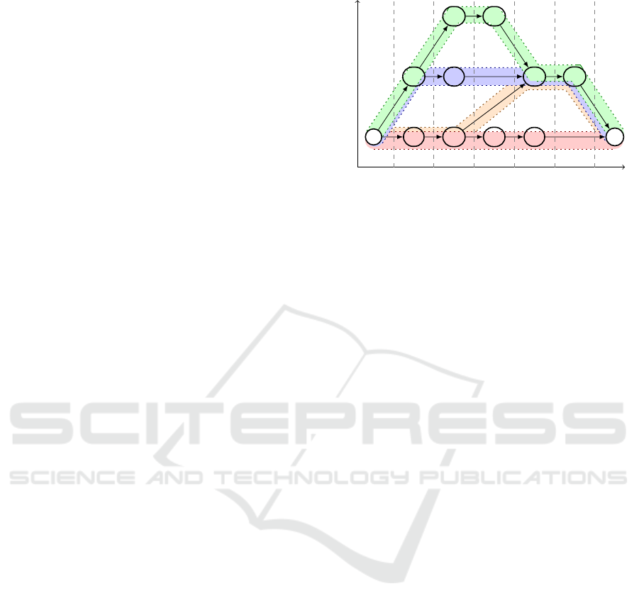
tance to s (Equation 1); see Fig. 2 for an example.

The level of a vertex can also be deﬁned in a recur-

sive way (Equation 2). The recursive deﬁnition yields

BIOINFORMATICS 2021 - 12th International Conference on Bioinformatics Models, Methods and Algorithms

an iterative method to calculate the levels of all ver-

tices, which we will use in our algorithms. For the

rest of the paper, we call level(v) the level of v.

level(v) = max{|P| : P = (s, ...,v) is a path in G}

(1)

level(v) =

(

0 v = s

max({level(u)|(u,v) ∈ E}) + 1 v 6= s

(2)

2.3 Minimum Path Cover Problem

(MPCP)

A path cover PC = {P

,..., P

} of a DAG G = (V, E) is

a set of paths, so that each vertex v ∈ V is part of a path

∈ PC. The size of a path cover PC is deﬁned as the

number of paths in PC. Since a single vertex deﬁnes a

path, V itself is a path cover of size |V |. The minimum

path cover problem is the problem of ﬁnding a path

cover PC of minimum size p

∗

. The minimum size p

∗

is called the width of G.

3 COORDINATE SYSTEM FOR

ACYCLIC NUCLEOTIDE

GRAPHS

To identify a locus in the pangenome, we need a coor-

dinate for each vertex of the nucleotide graph. In this

paper, we propose a new coordinate system for nu-

cleotide graphs that meets the requirements of mono-

tonicity, readability, and (horizontal and vertical) spa-

tiality. The coordinate of a vertex v in our new co-

ordinate system is a pair of two integers. The ﬁrst

component of the coordinate is the level of vertex v

in the DAG, which measures the distance from the

source to v. The second component is an identiﬁer

of a path to which v belongs. In order to use as few

path identiﬁers as possible, we will solve the mini-

mum path cover problem. In what follows, we elabo-

rate on this idea and provide an algorithm that gener-

ates such a coordinate system. For technical reasons,

we deal with DAGs that have a unique source s and

a unique sink t (the only vertices with in-degree and

out-degree 0, respectively). Graphs without a unique

source or sink can be modiﬁed by adding a super

source s and a super sink t to V , plus edges from s

to all former sources and edges from all former sinks

to t; see Fig. 2. In a graph with a unique source and

sink every vertex lies on some path from the source

to the sink and every path can be extended to a path

from s to t. Hence, there is always a minimum path

T G C

A GA T

G G

level

1 2

5 6

path

(0,1) (1,1) (2,1) (3,1)

(4,2) (5,2)(1,2) (2,2)

(2,3) (3,3)

(4,1) (6,1)

Figure 2: Nucleotide graph with super source and sink,

which represents the sequences TGCT, TGAG, ATAG and

AGGAG. The set {P

} is not a minimum path

cover, but {P

} is. The paths in this ﬁgure all start

at s and end at t.

cover that solely consists of paths from s to t. If ` is

the length of the longest path in the nucleotide graph

G and PC

∗

= {P

,..., P

∗

} is a minimum path cover

of G (w.l.o.g. all paths in PC

∗

start at s and end at t),

then the coordinates of s and t will be (0, 1) and (`,1)

respectively and the coordinates of all other vertices

are elements of {1, ..., ` − 1} × {1, ..., p

∗

}. For a ver-

tex v ∈ V and a path cover PC, we denote the set of

all paths that include v by PC(v). One of the paths in

PC(v) is chosen to be the representative of v. A possi-

ble choice is the path with lowest id, hence the coordi-

nate of a vertex v is (level(v), min(PC

∗

(v))). Figure 2

depicts a DAG with a path cover and the coordinates

of its vertices.

The two coordinates can be thought of as a hor-

izontal and a vertical coordinate. The horizontal

coordinate—similar to the coordinate in a linear ref-

erence genome—is the offset to the start of the chro-

mosomal DNA sequences. The vertical coordinate is

a path identiﬁer, which can be chosen in such a way

that it carries useful information. For example, one

could assign the vertices of the most likely genome

(the reference) to the path with id 1, the vertices of

the second most likely haplotype to the path with id

2, etc.

Moreover, this coordinate system satisﬁes the cri-

teria mentioned above. Having only two coordinates,

which both carry useful information, can be called

’readable’. Monotonicity follows directly from the

use of the level function in the ﬁrst coordinate: the

genome graph coordinates of successive bases within

a genome are increasing. Finally, the coordinate sys-

tem also meets the requirement ’spatiality’. If two

vertices represent a variant of each other, for instance

a SNP, then they will be at the same level and share

their ﬁrst coordinate. Thus, we have vertical spatial-

Coordinate Systems for Pangenome Graphs based on the Level Function and Minimum Path Covers

ity. Two vertices that represent nucleotides that are

close to each other in the genome will be at levels

close to each other. If they belong to the same haplo-

type, they will be covered by the same path. In this

way, horizontal spatiality is achieved.

To generate such a coordinate system, we calcu-

late the level of each vertex and solve the MPCP. The

coordinate of a vertex can then easily be reported as

a combination of its level and the identiﬁer of a path

that covers it.

4 SOLVING THE MPCP

The classical solution of the MPCP works as follows.

The MPCP is reduced to a maximum cardinality bi-

partite matching problem, which in turn is reduced to

a maximum ﬂow problem; see Cormen et al. (2009).

Since the latter can be solved by the Ford-Fulkerson

method, this method can also solve the MPCP. This

approach takes O (n

) time (in this paper we assume

|V | = n and |E| = m).

akinen et al. (2015) described a different

method to solve the MPCP. They reduced this prob-

lem ﬁrst to a minimum cost ﬂow problem, and then

to a minimum cost circulation problem. Overall, their

solution takes O(nm + n

log(n)) time.

Kuosmanen et al. (2018) introduced an algo-

rithm that ﬁrst generates an initial solution by us-

ing a method based on a classical greedy set cover

algorithm and then optimizes that solution with a

ﬂow algorithm. They showed that the initial path

cover has the size p ≤ p

∗

log(n), where p

∗

is the

width of the DAG. Therefore, their algorithm runs in

O(m p

∗

log(n)) time.

We will use a method comparable to the latter.

First, an initial path cover PC of size p will be cal-

culated in O(p m) time using a heuristic algorithm.

Then a network ﬂow algorithm, which makes use of

the Ford-Fulkerson method, is employed to reduce

the path cover to minimum size. A description of

the network ﬂow algorithm can be found in Kuosma-

nen et al. (2018, Section 2) and will not be repeated

here. Minimizing the ﬂow takes O ((p − p

∗

)m) time

because ﬁnding and adding a ﬂow requires O (m) time

and p− p

∗

ﬂows will be added. To report a path, O(m)

time is needed. Since there are p

∗

paths, reporting all

paths takes O(p

∗

m) time. In total, our method gener-

ates a minimum path cover in O (pm) time, where p

is the size of the initial path cover.

Algorithm 1: Calculate an initial path cover. An entry

path[i] in the array path is a list of all vertices that are

contained in path i.

Data: DAG G = (V,E) with source node s,

a vector d

of size |V | containing the

in-degree of each node

Result: An array level of size |V | containing the

level of each node, a set R

for each node

v, which contains all candidate paths for v.

1 level[s] ← 0

2 l ← 0, Q

← {s}, Q

l+1

←

3 p ← 0

4 while Q

0 do

5 for v ∈ Q

/* choose a path to cover v */

6 R

←

7 for (u, v) ∈ E do

8 for i ∈ R

9 last ← last element of path[i]

10 if level[last] < level[u] ∨ last = u

then

11 R

← R

∪ {i}

12 if R

0 then

/* add a new path */

13 p ← p + 1

14 R

← {p}

15 path[p] ← [v]

16 else

/* the path min(R

) is chosen

to cover v */

17 i ← min(R

)

18 ﬁnd the path P from the last node of

path i to v

19 append P to path[i]

20 for (v, w) ∈ E do

21 d

[w] ← d

[w] − 1

22 if d

[w] = 0 then

23 level[w] ← l + 1

24 Q

l+1

← Q

l+1

∪ {w}

25 l ← l + 1

26 Q

← Q

l+1

27 Q

l+1

←

4.1 Generating an Initial Path Cover

Algorithm 1 generates an initial path cover. It tra-

verses the graph level-wise from s to t and the path

cover is computed iteratively by extending the cur-

rent partial path cover to the next level. At level 0 the

source vertex s is covered by path 1. While visiting

the vertices of level l, the vertices of level l + 1 are

calculated. Furthermore, the algorithm tries to cover

all vertices of level l by extending paths that end at a

level < l with a vertex of level l. If no suitable path

can be found for a vertex, the algorithm will add a

BIOINFORMATICS 2021 - 12th International Conference on Bioinformatics Models, Methods and Algorithms

new path. In the following, it will be explained how

the level of a vertex is calculated and afterwards how

the path cover is generated.

The array level stores the level of each vertex v,

i.e. level[v] = level(v). The queue Q

contains all ver-

tices of level l. Initially l is 0, Q

= {s} and level[s] =

0 because the source is the only vertex in level 0. Fur-

thermore, there is an array d

, which initially stores

the number of incoming edges for each vertex. When

a vertex v at level l is encountered, d

[w] is decre-

mented by one for each successor w of v. If d

[w] = 0,

then all predecessors of w have been visited before.

In this case, level(w) = level(v) + 1 = l + 1 because

v has highest level among all the predecessors of w.

Lines 23-24 of Algorithm 1 handle this case by set-

ting level[w] = l + 1 and adding w to the queue Q

l+1

When all vertices of level l have been dealt with, the

algorithm will start the next iteration with the vertices

of the level l + 1 (lines 25-27). With this method, the

vertices are visited level by level. We now explain

how the algorithm covers the vertices with paths.

The counter p stores the number of paths used so

far (upon termination, p is the size of the path cover)

and for each path identiﬁer i, 1 ≤ i ≤ p, there is a

list of vertices path[i] in the array path. In the ﬁrst

iteration, the algorithm will add the path path[1] = [s].

This means that the ﬁrst path consists of the vertex s.

Moreover, the algorithm calculates a set R

for

each vertex v, which contains the identiﬁers of all

candidate paths for v, i.e. all paths that can poten-

tially cover v. A path that covers v must be selected

from this set R

. In the following, we choose min(R

)

to be that path. A condition for a path i to be in

is that i was a candidate for a predecessor u of v

i.e. i ∈ R

. It follows as a consequence that R

is a

subset of

(u,v)∈E

, but in general the sets are not

equal. For example, a path i ∈

(u,v)∈E

might have

already been used to cover a vertex w 6= v at level

l = level(v). We use a case distinction to ﬁnd the can-

didate paths. Let i ∈ R

, where u is a predecessor of

v, and let last be the last element of path[i]. If (a)

level[last] < level[u], then i was a candidate path for

u that was neither chosen to cover u nor one of its suc-

cessors. Hence it is a candidate path for v. If (b) path i

ends at u (i.e. last = u), then i is also a candidate path

for v.

Algorithm 1 calculates R

by the case distinction

described above (lines 8-11). If R

is empty after this

step, none of the existing paths can be used to cover

v. In this case, the algorithm adds a new path with

identiﬁer i

new

= p + 1 and uses this to cover v (lines

13-15). Otherwise, if R

is non-empty after this step,

the path with identiﬁer i = min(R

) is chosen to cover

v and path[i] is updated accordingly (lines 17-19). To

this end, one must ﬁnd a path P (implemented as a list

of vertices) from the last vertex last of path i to v. This

is done be tracing a path from v back to last. Initially,

the list P just contains v. Then vertices are added at

the front of the list until the vertex last is reached.

A vertex u can extend the path P at the front if (a)

it is a predecessor of the current front, (b) i ∈ R

, and

will ultimately reach last because the condition at line

10 of Algorithm 1 ensures that, among all vertices at

level level(last), only last can propagate the path i.

Upon termination of Algorithm 1, the paths in ar-

ray path form a path cover. However, we are solely

interested in paths from s to t. In what follows we

explain Algorithm 2, that extends the paths on both

ends. Let v

and v

be the ﬁrst and the last vertex of

path[i], respectively. We have to add a subpath from s

to a predecessor of v

and a subpath from a successor

of v

to t to obtain a path from s to t. We can ﬁnd

such subpaths by a depth ﬁrst search in linear time, or

we can copy them from other paths. Note that path

1 is a path from s to t already, since 1 is the smallest

path identiﬁer and will therefore be used continuously

from vertex s to t. For i 6= 1 all predecessors of v

are covered by paths < i because v

is the ﬁrst vertex

covered by a path ≥ i. Likewise, all successors of v

are covered by paths < i because i was not chosen to

cover one of them. These observations lead to an it-

erative process for ﬁnding the subpaths that shall be

copied. When extending path i, all paths < i are paths

from s to t. Among all predecessors u of v

, we select

the one that is covered by the path with the smallest

identiﬁer j. Since j < i, j is a path from s to t and we

can copy the subpath from s to u. In the same way, we

can ﬁnd a path from a successor of v

to t. Algorithm

2 extends each path to be a path from s to t.

Algorithms 1 and 2 compute an initial path cover

in O(p m) time, where p is the size of the cover and

m is the number of edges in the DAG. This is because

every edge is considered exactly once in line 7 of Al-

gorithm 1 and the loop in line 8 of Algorithm 1 is

iterated at most p times. Moreover, the overall time

required by line 18 of Algorithm 1 and Algorithm 2

is also O(p m) because for each of the p paths each

edge is considered at most once. (If one wants to cal-

culate the minimum path cover as described above,

one could directly insert ﬂow into the ﬂow network

instead of storing and reporting a path.)

4.2 A Simple Heuristic

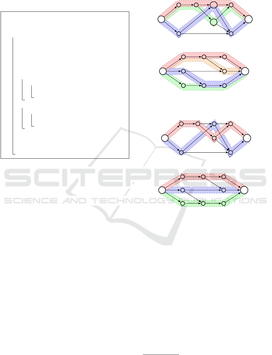
In general, Algorithms 1 and 2 do not deliver a mini-

mum path cover; see Fig. 3. This is because the order

in which vertices are covered by paths plays a key

Coordinate Systems for Pangenome Graphs based on the Level Function and Minimum Path Covers

Algorithm 2: After iteration i, path[i] is a path from s

to t. Since j and k must be smaller than i, these paths

are already paths from s to t.

Data: DAG G = (V, E), path array path and can-

didate sets R

after applying Algorithm 1

Result: Path array path contains paths from s to t

1 for i ← 2 to p do

/* path 1 is already a path from s to t

2 j,k ← ∞

3 u

← ⊥

4 v

← ﬁrst element of path[i]

5 v

← last element of path[i]

6 for (u,v

) ∈ E do

7 if min(R

) < i then

8 u

← min(R

)

9 u

← u

10 for (v

,u) ∈ E do

11 if min(R

) < k then

12 k ← min(R

)

13 u

← u

14 Prepend the vertices of the subpath from s to u

of path[ j] to path[i]

15 Append the vertices of the subpath from u

to t

of path[k] to path[i]

role. For example, in level 3 of the graph depicted

in Fig. 3.a, the vertices u and v must be covered with

paths. The candidate paths for vertex u are 1 and 2,

whereas only path 1 reaches vertex v. Algorithm 1

will ﬁrst cover vertex u with path 1 because this is the

smallest candidate (i.e. min(R

) = 1). It follows that

vertex v cannot be covered by path 1 and consequently

a new path 3 must be added to cover this vertex. A

better solution would be to cover vertex u with path

2 and vertex v with path 1, as shown in Fig. 3.c. It is

possible to improve the size of an initial path cover (in

many cases) by modifying the way in which a path is

chosen to cover a vertex (i.e. it is not necessarily the

path with identiﬁer i = min(R

)).

To get a locally optimal solution (i.e. an optimal

solution for a ﬁxed level l), we could solve a maxi-

mum cardinality bipartite matching problem. Deﬁne

a bipartite graph as follows. Let X be the set of all

vertices in Q

and let Y be the set Y =

v∈X

. Fur-

thermore, there is an edge between v ∈ X and i ∈ Y

if and only if i ∈ R

. Now the problem is to ﬁnd a

maximum cardinality matching in the bipartite graph,

i.e. a matching that contains the largest possible num-

ber of edges. However, the example in Fig. 3.b and

3.d shows that the locally optimal solutions do not

yield a globally optimal solution. This is because one

of the two solutions to the maximum cardinality bi-

partite matching problem at level 2 in Fig. 3.b would

cover the upper vertex with path 1 (the only possi-

bility) and the lower vertex with path 2. In level 3,

Calculated path cover:

{1}

{2}

{1} {1,2}

{3}

{1,3}

{2,3}

{1,2,3}

{1}

{2}

{3}

{1}

{2,3}

{1}

{4}

{2,3}

{1,2,3,4}

Minimum path cover:

{1}

{2}

{1} {2}

{1}

{2}

{1,2}

{1}

{2}

{3}

{1}

{3}

{1}

{2}

{3}

{1,2,3}

Figure 3: Different examples of path covers. For each ver-

tex v, the set R

is shown below v. The path covers depicted

in a) and b) are calculated by Algorithms 1 and 2, whereas

c) and d) show the corresponding minimum path covers.

however, it becomes clear that a globally optimal so-

lution (a minimum path cover) can only be obtained

if the lower vertex at level 2 is covered with path 3.

Since the computation of locally optimal solutions

is time-consuming and does not yield a globally op-

timal solution anyway, we will use a simple heuristic

to obtain local solutions. In each level l, we use a

bucket sort to sort the vertices v in Q

in increasing

order by the number of candidate paths (the cardinal-

ity of R

). Then we process the vertices v in that order

as follows:

1. If R

is empty, assign a new path to v and continue

with the next vertex.

2. Otherwise, take the ﬁrst element i from R

In our implementation R

is implemented as an ordered

set and the elements are processed in that order.

BIOINFORMATICS 2021 - 12th International Conference on Bioinformatics Models, Methods and Algorithms

• If i was already used to cover another vertex at

the current level, remove i from R

and continue

at (1).

• Otherwise, assign i to v and continue with the

next vertex.

The intuition behind this procedure is simple. For a

singleton set R

= {i}, there is no choice: we must

assign i to v. Once we have done this, i cannot cover

another vertex from Q

, but a vertex u with a big can-

didate set R

has more options than v. Thus, if we

start with small candidate sets, there is a fair chance

that a big candidate set R

still contains a path that can

be assigned to u when it is u’s turn.

5 EXPERIMENTAL RESULTS

We implemented the algorithms described above and

built a prototype, that generates a coordinate sys-

tem for a DAG. The software and scripts to replicate

the experiments are available at: www.uni-ulm.de/

in/theo/research/seqana. The program takes a graph

in GFA format as input, computes a path cover and

the corresponding coordinate system, and outputs the

graph (in which vertices are aligned with their coor-

dinates) in DOT format.

Three different strategies were used to compute an

initial path cover:

• the greedy set cover method (gsc) proposed by

Kuosmanen et al. (2018),

• our level-wise computation of the cover (lev), and

• our simple heuristic (sh).

The calculation of the minimum path cover was tested

with real world data and generated data. All experi-

ments were conducted on a Ubuntu 16.04.4 LTS sys-

tem with two 16-core Intel



Xeon



E5-2698 v3 pro-

cessors and 256 GB RAM.

We used the variation graph toolkit vg (Gar-

rison et al., 2018) to construct a graph from the

FASTA

and VCF

ﬁles for the ﬁrst human chromo-

some provided by the 1000 genome project (The 1000

Genomes Project Consortium, 2015). In vg, vertices

are not labeled with single nucleotides (as required

here), but with nucleotide sequences. That is why our

program replaces each vertex in the vg graph by a path

of vertices with nucleotides as labels. The resulting

graph has more than 255 ×10

vertices and 262 ×10

Available at: ftp://ftp.1000genomes.ebi.ac.uk/vol1/ftp

/technical/reference/phase2 reference assembly sequence/

Available at: ftp://ftp.1000genomes.ebi.ac.uk/vol1/ftp

/release/20130502/

edges. Since the graph has a relatively simple struc-

ture, all three strategies deliver an initial path cover

of size 9 and the initial path cover is a minimum path

cover already. Using the gsc strategy, the overall cal-

culation of the coordinates takes 48 min. The other

strategies lev and sh require 64 and 94 min, respec-

tively.

To get more complex graphs, we generated graphs

in two different ways. The ﬁrst method is inspired

by the well-known Erdos-Renyi model (Erd

os and

enyi, 1959) in which a graph is chosen uniformly

at random from the collection of all graphs which

have n vertices and m edges. We modiﬁed the model

in such a way that acyclic graphs with a unique

source and sink are generated. The set of vertices

is V = {1, . . . ,n} and the set of edges E initially is

{(1,u), (u, n)|u ∈ {2, . .. , n − 1}}. This ensures that 1

is the unique source and n is the unique sink. Then

two vertices u and v are chosen uniformly at random

from V \ {1, n}. If u < v then (u, v) is added to E, if

v < u then (v, u) is added to E, and if u = v no edge

is added to E. This process is repeated until the graph

contains m edges.

Our second method tries to generate pangenome

graphs that are more complex than the currently avail-

able pangenome graphs (as the one described above).

The parameters of this model are the number n of ver-

tices, a maximum size p for a path cover, and a path

length `. Again, V is {1, . . ., n}. The set of edges

E is a union of the edges of p generated paths. The

ﬁrst p − 1 paths are generated by choosing `+1 (pair-

wise different) vertices from {2,... , n − 1} uniformly

at random.

The ` + 1 vertices are then sorted in increasing or-

der, say u

< · ·· < u

`+1

. Finally, the edges (1,u

i+1

) for 1 ≤ i ≤ `, and (u

`+1

,n) are added to E.

The last path initially contains all vertices of V that

are not part of any of the previous paths. If this path

smaller than `, randomly chosen vertices are added

to the path until it has the length ` (depending on the

parameter, the last path can be signiﬁcant longer than

`). This generates a DAG with the unique source 1

and the unique sink n. Furthermore, it is clear that the

width of the graph is at most p.

We generated 200 graphs with each model. In the

Erdos-Renyi model, we used n = 10

vertices and be-

tween 2 × 10

and 4 × 10

edges. The number of lev-

els in the generated graphs varied between 420 and

830. In our second model, the parameter for the num-

ber of vertices was also n = 10

. The number of paths

was varied between 100 and 200 and the path length

was varied between 5,000 and 10,000. The graphs

generated in this way have between 1×10

and 2×10

edges and between 150,000 and 600,000 levels.

Coordinate Systems for Pangenome Graphs based on the Level Function and Minimum Path Covers

Size of initial path cover Time for generating

the coordinate system

0 100 200

p∗

lev

gsc

100

150

200

lev

gsc

sec.

0 100 200

p∗

lev

gsc

0 100 200

lev

gsc

sec.

0 10

p∗

lev

gsc

min

0 30

90 120

lev

gsc

min.

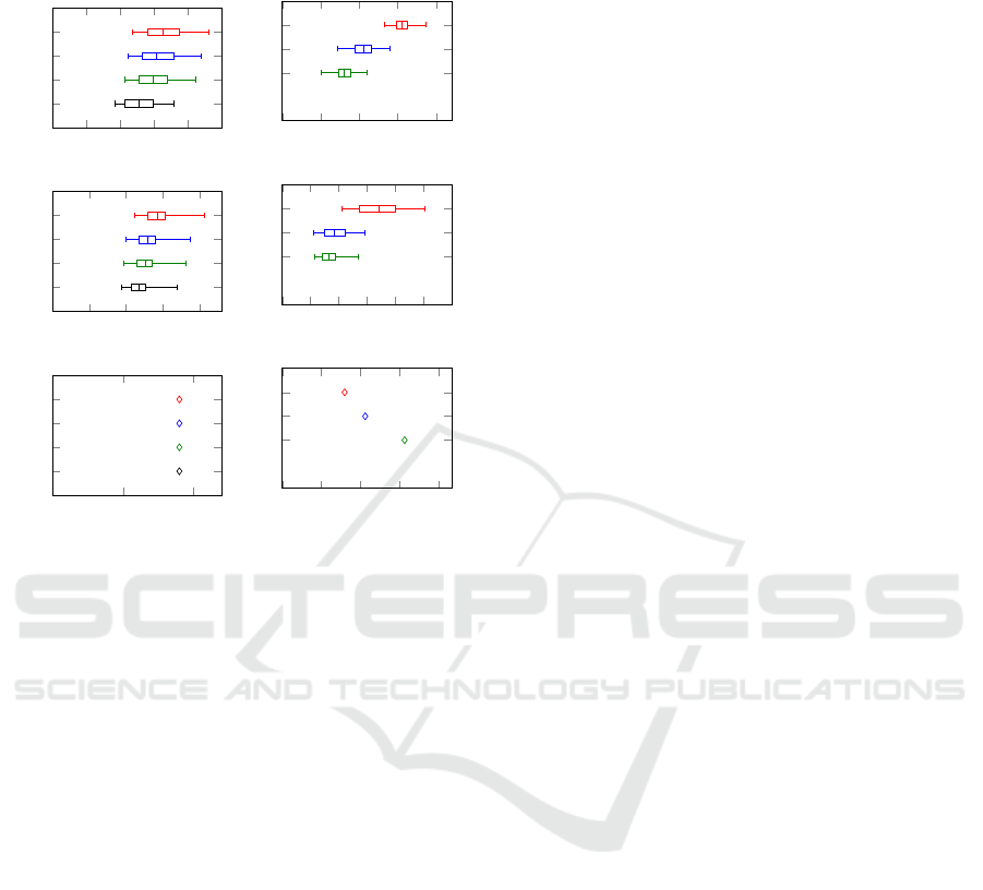
Figure 4: Comparison of the different approaches: the

greedy set cover (gsc), our level-wise computation of the

cover (lev), and our simple heuristic (sh). On the top:

graphs generated by the Erdos-Renyi model. In the middle:

graphs generated by the second model. On the bottom: the

graph generated from real world data using the vg toolkit.

Recall that p

∗

denotes the width of the graph (the size of a

minimum path cover).

In our experiments, we measured the size of the

initial solution and the time to calculate the coordi-

nate system (this includes the time for ﬂow minimiza-

tion). The distributions of the measured values are

shown in Figure 4. It can be seen that our method

calculates smaller initial path covers than the greedy

set cover strategy and that the simple heuristic further

improves the result. To be more precise, in each of

the 400 test cases, the initial path cover constructed

by our strategy was smaller compared to that gen-

erated by greedy set cover strategy. Furthermore, in

98% of the test cases the simple heuristic sh returned

a smaller initial path cover than the lev method. We

would like to stress that the overall run-time strongly

depends on the time required for ﬂow minimization,

i.e. the smaller the initial path cover the better. That

is why the simple heuristic outperforms the other ap-

proaches in most cases. However, the cost of using the

simple heuristic cannot be compensated by the faster

ﬂow minimization in all cases.

6 DISCUSSION

In this paper, we proposed a new coordinate system

for acyclic nucleotide graphs, which meets the re-

quirements monotonicity, readability as well as hor-

izontal and vertical spatiality. The ﬁrst part of the

coordinate is the level of a vertex, which in essence

is the offset from the start of the genomic sequence

(chromosome). The second part is a path identiﬁer,

which can be interpreted as a vertical coordinate. By

using a minimum path cover, the number of path iden-

tiﬁers is reduced to a minimum, which leads to more

comprehensible coordinates.

The minimum path cover can be calculated by an

algorithm that ﬁrst ﬁnds an initial solution and then

transforms this solution into a minimum path cover.

The run-time of the algorithm strongly depends on

the quality of the initial solution. Our algorithm sh

generates the smallest initial solutions. The lev strat-

egy is the fastest in ﬁnding an initial solution in the

generated graphs. In graphs with low width p

∗

, such

as the graph constructed by vg using a FASTA and

VCF ﬁle, the gsc strategy is faster. Since all strate-

gies are already ﬁnding minimum solutions in such

graphs, the initialization, instead of the minimization,

is the crucial step. Therefore, using the gsc strategy is

best for the tested real world data. In more complex

graphs, the strategy sh is superior.

It should be investigated how additional informa-

tion like haplotypes or frequency of alleles can be in-

corporated into the second coordinate, because this

would make the coordinate systems even more infor-

mative.

ACKNOWLEDGEMENTS

Funding: This work was supported by the DFG (OH

53/7-1).

REFERENCES

Consortium, I. H. G. S. (2001). Initial sequencing and anal-

ysis of the human genome. Nature, 409:860–921.

Consortium, T. C. P.-G. (2016). Computational pan-

genomics: status, promises and challenges. Brieﬁngs

in Bioinformatics, 19(1):118–135.

Cormen, T. H., Leiserson, C. E., Rivest, R. L., and Stein,

C. (2009). Introduction to Algorithms. MIT Press,

Cambridge, MA.

Dilthey, A., Cox, C., Iqbal, Z., Nelson, M. R., and McVean,

G. (2015). Improved genome inference in the mhc

using a population reference graph. Nature Genetics,

47(6):682–688.

BIOINFORMATICS 2021 - 12th International Conference on Bioinformatics Models, Methods and Algorithms

Erd

os, P. and R

enyi, A. (1959). On random graphs. Publi-

cationes Mathematicae, 6:290–297.

Garrison, E., Sir

en, J., Novak, A. M., Hickey, G., Eizenga,

J. M., Dawson, E. T., Jones, W., Garg, S., Markello,

C., Lin, M. F., et al. (2018). Variation graph toolkit

improves read mapping by representing genetic varia-

tion in the reference. Nature biotechnology.

Kuosmanen, A., Paavilainen, T., Gagie, T., Chikhi, R.,

Tomescu, A., and M

akinen, V. (2018). Using min-

imum path cover to boost dynamic programming on

dags: Co-linear chaining extended. In Raphael, B. J.,

editor, Research in Computational Molecular Biology,

pages 105–121, Cham. Springer International Pub-

lishing.

akinen, V., Belazzougui, D., Cunial, F., and Tomescu,

A. I. (2015). Genome-scale algorithm design. Cam-

bridge University Press.

Paten, B., Novak, A. M., Eizenga, J. M., and Garrison, E.

(2017). Genome graphs and the evolution of genome

inference. Genome Research, 27(5):665–676.

Rand, K. D., Grytten, I., Nederbragt, A. J., Storvik, G. O.,

Glad, I. K., and Sandve, G. K. (2017). Coordinates

and intervals in graph-based reference genomes. BMC

Bioinformatics, 18(1):263.

The 1000 Genomes Project Consortium (2015). A global

reference for human genetic variation. Nature,

526:68–74.

Coordinate Systems for Pangenome Graphs based on the Level Function and Minimum Path Covers