
A Function Dependency based Approach for Fault Localization with D
∗
Arpita Dutta
a
and Rajib Mall
b
Indian Institute of Technology Kharagpur, India
Keywords:
Function Dependency Graph, Fault Localization, Comprehensibility, Program Analysis, Debugging.
Abstract:
We present a scheme for hierarchically localizing software faults. First the functions are prioritized based on
their suspiciousness of containing a fault. Further, the bug is localized within the suspected functions at the
specific statement level. In our approach, a new function dependency graph is proposed, and based on that
function prioritization is performed. In order to differentiate between the functions with equal suspiciousness
value, function complexity metrics are considered. We proposed two different dependency edge weighting
techniques, viz., Distribution Specified Normalization (DSN) method, and Highest Weight Normalization
(HWN) method. These techniques help to measure the relevance of an edge in propagating a fault. We use
spectrum-based fault localization (SBFL) technique DStar(D
∗
) to localize the bugs at the statement level.
We also extended our approach to localize multiple fault programs. Based on our experimental results, it is
observed that using DSN and HWN scoring schemes, there is a reduction of 43.65% and 38.88% of statements
examined compared to the well-accepted SBFL technique DStar(D
∗
) respectively.
1 INTRODUCTION
With the increasing size and complexity of software
systems, bugs are inevitable. Advancements in soft-
ware development techniques and testing practices
help to detect most of the faults in early stages of soft-
ware life cycle (Mall, 2018). However though few
remain, and numerically these are substantial consid-
ering the size of the program. Debugging is a time-
consuming and effort-intensive activity. Bug local-
ization is the most vital task during debugging. Tech-
niques that can minimize the effort and time required
to localize the bugs can help to reduce the overall cost
of development and also enhance the quality of the
software (Wong et al., 2016). In the past two-to-three
decades, various fault localization (FL) techniques are
reported in the literature (Liu et al., 2005; Abreu et al.,
2009; Ascari et al., 2009; Feng and Gupta, 2010;
Wong et al., 2013; Wong et al., 2016; Yu et al., 2017;
Spinellis, 2018; Ardimento et al., 2019; Dutta et al.,
2019; Thaller et al., 2020).
Weiser (Weiser, 1984) proposed the concept of
program slicing. A program slice contains list of
statements that effects the value of a variable at a
specific location of program. Later, Agrawal et al.
(Agrawal and Horgan, 1990) extended their approach
a
https://orcid.org/0000-0001-7887-3264
b
https://orcid.org/0000-0002-2070-1854
by adding the execution-time information of test in-
puts and named their approach as dynamic slicing.
Dynamic slicing helps to minimize the search space
as compared to the static slicing. Program spectrum-
based fault localization (SBFL) techniques are re-
ported as both effective and efficient (Wong et al.,
2013; Liu et al., 2005; Wong et al., 2016). Initially,
SBFL approaches considered only failed test case in-
formation (Korel, 1988), but they were shown to be
ineffective (Agrawal et al., 1995). Later, Jones et
al. (Jones and Harrold, 2005) proposed an executable
statement hit spectrum based FL approach to increase
the effectiveness of the SBFL schemes. Wong and
colleagues (Wong and Qi, 2009; Wong et al., 2010)
and Dutta et al. (Dutta et al., 2019) reported neural
network models for the same.
Several fault localization techniques have become
popular, but these techniques are time-consuming and
ineffective for large-size programs. Even for small
programs, these techniques require to examine 40%-
45% of program code. Our objective is to develop an
FL technique which requires fewer number of state-
ment examination as compared with the contempo-
rary fault localization methods.
For a given source program, we firstly define
a Function Dependency Graph (FDG). This graph
is generated by obtaining data, control, and inter-
procedural dependencies from an equivalent control
Dutta, A. and Mall, R.
A Function Dependency based Approach for Fault Localization with D*.
DOI: 10.5220/0009769402730283
In Proceedings of the 15th International Conference on Software Technologies (ICSOFT 2020), pages 273-283
ISBN: 978-989-758-443-5
Copyright
c
2020 by SCITEPRESS – Science and Technology Publications, Lda. All rights reserved
273

flow graph (CFG) of the same program. We further
assign weights to the dependency edges of the FDG
based on their contribution in propagating a fault.
The value of assigned weights to the dependencies
are computed using the coverage information of the
failed and passed test cases. We reported two dif-
ferent schemes Distribution Specified Normalization
(DSN) and Highest Weight Normalization (HWN) to
calculate the weights of the dependency edges. Sub-
sequently, the nodes of the FDG are prioritized based
on their suspiciousness values and function compre-
hensibility measure. The hierarchical procedure helps
to reduce the search space to the top most suspicious
functions only. Then, existing spectrum-based FL
technique DStar(D
∗
) is used to prioritize the state-
ments of obtained set the most suspicious functions.
The remaining sections of the paper are written as
follows: first, we present the basic concepts in Section
2. Subsequently, the proposed approach is explained
in Section 3. The experimental setup and obtained
results are discussed in Section 4. Section 5, presents
the extension of our proposed approach to handle pro-
grams with multiple faults. Threats to the validity of
experimental results are discussed in Section 6. We
present a comparison with related works in Section 7.
Lastly, we conclude our work in Section 8.
2 BASIC CONCEPTS
This section presents few important definitions which
are essential to understand our work.
• Program Dependency Graph (PDG). For a pro-
gram P, PDG is represented as G
p
=(V, E), where
V is the set of nodes representing statements of P
and E is the set of control and data dependency
edges (Mund G. B., 2007).
• System Dependency Graph (SDG). The SDG
for a program P is represented as G
s
=(V, E),
where V is the set of nodes representing state-
ments of P and E is the set of edges represent
the control, data, and inter-procedure dependen-
cies among the statements (Mund G. B., 2007).
• Weighted System Dependency Graph
(WSDG). A WSDG is primarily a system
dependency graph in which all the dependency
edges ( Data, Control, and Inter-procedure) have
weights linked with them (Deng and Jones,
2012).
• Comprehensibility. The facileness with which a
code segment can be understood is called its com-
prehensibility (Miara et al., 1983). It is inversely
proportional to the code block complexity. If a
code segment is complex and challenging to un-
derstand, then it has a higher possibility of bug
containment.
• DStar(D
∗
). It is a executable hit spectrum based
based FL technique reported by (Wong et al.,
2013). DStar uses a modified form of Kulczynski
coefficient (Choi et al., 2010). In this method, the
suspiciousness score of statement s is calculated
using Equation 1.
susp(s) =
(s
e f
)
∗
s
ep
+ s
n f
(1)
where, susp(s) shows the suspiciousness score of
statement s; s
e f
and s
ep
represents the number
of failed and passed test cases that have exer-
cised statement s. s
n f
shows the number of failed
test inputs that have not invoked the statement s.
DStar performs best for
∗
= 2, i.e., D
2
, in most of
the programs. The ‘
∗
’ is a numerical variable, and
it varies for different programs.
3 PROPOSED APPROACH: FDBD
∗
We named our proposed approach as FDBD
∗
. It is an
abbreviation for Function Dependency Based FL with
D
∗
.
In this work, a hierarchical method is used to re-
duce the search space and the time required to local-
ize a fault. We have assumed that a fault is propagated
by exercising various dependencies present in a pro-
gram, from an incorrect statement to the output. Each
time a test case executes, the bug present in a function
gets carried towards the called function by executing
some of the dependencies that exist between them.
The statements present in the functions invoked by the
failed test cases are called as Potential Contributors
for propagating a fault. On the other hand, the de-
pendencies executed by a successful test case are less
potential for propagating a fault. A PDG can model
a program with single function. However, in prac-
tice, a program contains multiple functions. An SDG
is used to represent a program with more than one
functions. But, it represents each instruction as a sin-
gle node. This results to a complex and huge graph,
even for a medium-size program. The space complex-
ity of an SDG is O(s + d) where, s and d represent
the statements presents in the program and dependen-
cies among the statements respectively. Therefore, it
becomes quite expensive to traverse the graph to lo-
calize the faulty instruction for large-size programs.
To solve this problem, we propose a Function Depen-
dency Graph (FDG). It presents a function level ab-
straction of SDG. FDG contains only the dependency
ICSOFT 2020 - 15th International Conference on Software Technologies
274
entry: main
entry: foo1
entry: foo
call: foo
call: foo1
1 2
3
4
5
6
7
8
9
actual-in and actual-
out arguments
formal-in and formal-
out arguments
calling node
for function
entry node
for function
edges available
in FDG
edges not
available in FDG
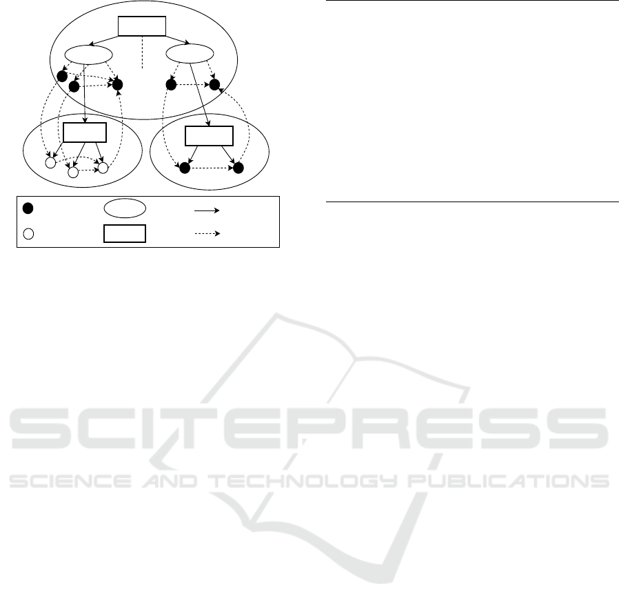
Figure 1: Function Dependency Graph.
information among functions and yields an efficient
way to localize the faults.
3.1 Function Dependency Graph (FDG)
Definition 1. An FDG for a program P is represented
as G = (N, E). It is a directed graph. The nodes in set
N represent the functions, and the edges in set E show
the dependencies exist among the nodes in set N.
Structure of an FDG. Every ordinary C-program
contains the main function and different other func-
tions. We represent each function with a specific en-
try node called FEN (Function Entry Node). FEN is
connected with three types of nodes (vertices). These
nodes are argument-in, argument-out, and call ver-
tices. Call vertex represents the call site of the func-
tion. Argument-in and -out vertices show the propa-
gation of data from the actual to formal parameters
and from formal to actual parameters, respectively.
These two vertices are control dependent on the con-
nected FEN. Values from the calling function are
copied to the argument-in parameters, and the func-
tion return values are copied back to the argument-out
parameters. Figure 1 represents the generated FDG
for the C-program shown in Figure 2.
3.2 Fault Localization with FDBD
∗
A fault is transmitted from the buggy function to-
wards the output by exercising different dependency
edges. We attach weights to the dependency edges
based on their probability of propagating a bug. The
weight attached to a dependency edge is computed by
the frequency that the edge is being exercised during
the propagation of fault towards the output of the pro-
gram. The weights of the dependency edges exercised
void main(){
int var_a, var_b;
var_a=0;
var_b=1;
var_c=foo(var_a, var_b);
var_d=foo1(var_a);
}
int foo(int var_a,int var_b){
var_a = var_a+var_b;
return var_a;
}
int foo1(int var_c){
return var_c+10;
}
Figure 2: Example C-program with three functions.
by failed test cases are multiplied by a factor that lies
in between 0 to 1. On the other hand, edges used by
passed test cases are multiplied with another factor
that is higher than 1. The dependency edges weights
are inversely proportional to their likelihood of prop-
agating a bug. Specifically, an edge with a higher
weight has less probability of participating in the fault
propagation.
3.2.1 Weighting Schemes for Dependencies
We first present some notations which we use in the
definition of two different dependency edge scoring
methods:
• P = Number of passed test cases present.
• F = Number of failed test cases present.
• P(i) = Total passed test cases that have invoked
the i
th
dependency edge (1 ≤ i ≤ n) and n is the
number of dependency edges in FDG.
• F(i) = Total failed test cases that have invoked the
i
th
dependency edge (1 ≤ i ≤ n) and n is the num-
ber of dependency edges in FDG.
1. Highest Weight Normalization Method(HWN): In
this method, two heuristic constants, w
pass
(w
pass
> 1)
and w
f ail
(0 < w
f ail
< 1) are used. With these two
constants, we calculate the weight that will be as-
signed to any dependency edge. At the very begin-
ning, weights of all dependency edges are initialized
with 1. For every pass test case, weight of all the in-
voked dependency edges are increased by multiplying
them with a factor w
pass
. In contrary, for the failed
test case, weights of the edges are reduced by multi-
plying them with factor w
f ail
. After the execution of
all test cases, the weight of a dependency edge can be
computed using Equation 2.
W (i) = (w
pass
)
P(i)
∗ (w
f ail
)
F(i)
(2)
A Function Dependency based Approach for Fault Localization with D*
275

where, W (i) presents the weight obtained by the i
th
dependency edge. Further, weights of the dependen-
cies are normalized with respect to the highest weight
value obtained by the considered set of dependency
edges using Equation 3.
NW (i) =
(W(i))
max(W(1), ...,W (n))
(3)
where, NW (i) and n represents the normalized weight
of dependency edge i and number of dependency
edges present in FDG, respectively.
2. Distribution Specified Normalization Method
(DSN): It is usually noticed that during the execu-
tion of a test suite, some of the dependency edges
are invoked in every execution. These edges are in-
voked by all the pass and the failed test cases. Assume
that there are 80% of fail and 20% of pass test cases
present in a test suite. Then, even if the edges are not
involved in propagating any fault, but they are com-
puted as suspicious for 80% of test cases. Here, the
weight attained by a dependency edge is dominated
by the factor w
f ail
over w
pass
.
To overcome the above-stated problem, we pro-
pose another dependency edge scoring scheme called
DSN. Our scheme considers the distribution of the
failed as well as the passed test cases for an exercised
dependency to assign the weight. In this method,
we use the previously determined factor w
f ail
(0 <
w
f ail
< 1) as it is. Whereas, we compute the value
of w
pass
based on the distribution of both failed and
passed test cases. The dependency edges that are in-
voked by every test input are known as unbiased de-
pendencies. We define some notations related to an
unbiased dependency:
1. PU(i): Number of pass test inputs which have ex-
ercised the i
th
unbiased dependency edge.
2. FU(i): Number of fail test inputs which have ex-
ercised the i
th
unbiased dependency edge.
With the above two notations, we compute the value
of factor w
pass
using Equation 4.
(w
pass
)
PU(i)
∗ (w
f ail
)
FU(i)
= 1
w
pass
= [
1
(w
f ail
)
FU(i)
]
1
PU(i)
(4)
By using these values for w
pass
and w
f ail
, we cal-
culate the weight of the rest dependencies using Equa-
tion 5:
W (i) = (w
pass
)
P(i)
∗ (w
f ail
)
F(i)
(5)
In the proposed DSN scheme, value of heuristic pa-
rameter w
pass
is required to be computed separately
for each program, unlike the HWN scheme. Further,
we normalize weights of all dependency edges with
Equation 3, and they have values in range of 0 to 1.
3.2.2 Prioritization of Functions
After the weight assigned to all the dependency edges,
the next step is to discover the potential contributors.
For this, we calculate the Fault Propagation score (FP-
score) of each FEN. FEN represents a function in
FDG. Hence, FP-score shows the suspiciousness of
a function for containing a fault. Dependencies enter-
ing and leaving into the function are liable for prop-
agating a fault. We take average of all the dependen-
cies connected with a FEN to calculate the FP-score,
as shown in Equation 6.
FP-score =
∑
i=m
i=1
NW (i) +
∑
j=n
j=1
NW ( j)
m + n
(6)
Where, m and n represents the number of incoming
and outgoing dependencies to an FEN. After assign-
ing weights to all the FENs, the resultant graph is
termed as a weighted dependency graph (WFDG).
3.2.3 Comprehensibility
Given a large-size program and a test suite, it is very
likely that many dependency edges end up with the
same weight. It results in a tie among multiple func-
tions. We considered the fact that complex function
has more chances of containing a fault, to break the
tie among different functions. We calculate the com-
plexity of each function. Because, it is widely ac-
cepted fact that complexity measure directly propor-
tional with the expected number of latent faults (Mc-
Cabe, 1976).
Let CF(i) be the complexity of i
th
function . We
use the following six metrics to calculate function
complexity: cyclomatic complexity, executable lines
of code (ELOC), count of parameters passed in func-
tion, total number of variables used, number of paths,
and maximum depth of nesting (if structure/ loops).
Each attribute is normalized using min-max normal-
ization using Equation 7 and their resultant values are
in between 0 to 1.
X
0
i j
=
X
i j
− X
min
j
X
max
j
− X
min
j
(7)
where, X
max
j
and X
min
j
are respective maximum and
minimum values for attribute j among all the func-
tions. X
0
i j
and X
i j
are the normalized and original
value of j
th
attribute of i
th
function. Further, we com-
pute comprehensibility of function i using Equation 8
with normalized attribute values.
CF(i) =
∑
k
j=1
X
0
i j
∑
n
i=1
∑
k
j=1
X
0
i j
(8)
where, k shows the count of attributes considered.
ICSOFT 2020 - 15th International Conference on Software Technologies
276
void print(int a, int b,int c){
printf("%d %d %d",a,b,c);
}
int add(int a, int b){
a = a + b;
return a;
}
int sub(int a, int b){
a = a * b;
return a;
}
void main(int argc, char **argv){
int a, b,c;
a = 0;
b = 0;
scanf("%d",&a);
if(a>=0){
b=2*a;
c=add(a, b);
print(a,b,c);}
else{
b=-1;
c=sub(a, b);
print(a,b,c);}
}
Figure 3: An example C-program.
3.2.4 Localization of Faulty Statements
After prioritizing the functions based on FP-Score and
comprehensibility, we examined the statements of the
functions in the top one-third of the suspected func-
tions list. To rank the statements of suspicious func-
tions, we adopted the SBFL technique DStar (Wong
et al., 2013). In the worst case, if the bug is not lo-
cated in the former set of functions, we search the bug
in the next one-third of the ranked list. The reason
behind choosing DStar is that it is state-of-the-SBFL
techniques (Wong et al., 2013).
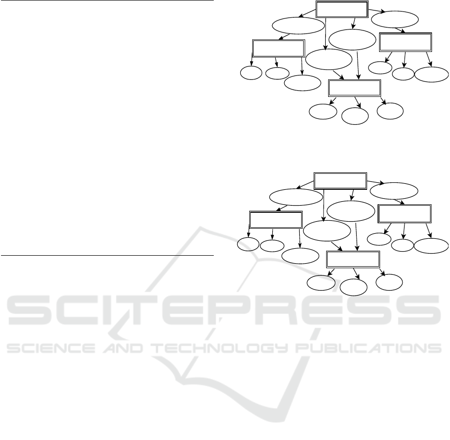
3.3 Example
In this section, we explain our proposed approach us-
ing an example C-program shown in Figure 3. As it
can be seen that the program contains four functions,
namely main(), add(), sub(), and print(). The
add() and sub() functions present add and subtract
operation respectively. The print() function prints
the values of parameters passed to it. The subtraction
function contain a bug i.e., in place of subtraction op-
erator, multiplication operator has been used.
Figure 4 shows the resultant Functional Depen-
dency Graph (FDG) for the example C-program
shown in Figure 3. Each dependency edge is marked
with its edge number and weight, separated with a
slash symbol. We use HWN (Highest Weight Nor-
malization) scoring scheme in this example. The
entry: main
entry: add
entry: print
entry: sub
call: add(a, b)
call:
print(a, b, c)
call:
print(a, b, c)
call: sub(a, b)
a=a_in b=b_in
c_out=a+b
a=a_in
b=b_in c_out=a*b
a=a_in
b=b_in
c=c_in
1/1 3/1
5/1
7/1
9/1
16/1
17/1
10/1
11/1
12/1
13/1
14/1
15/1
2/1
4/1
6/1
8/1
Figure 4: Function Dependency Graph(FDG) for the C-
program of Figure 3 with initial weights of all dependency
edges initialized to 1.
entry: main
entry: add
entry: print
entry: sub
call: add(a, b)
call:
print(a, b, c)
call:
print(a, b, c)
call: sub(a, b)
a=a_in
b=b_in
c_out=a+b
a=a_in
b=b_in c_out=a*b
a=a_in
b=b_in
c=c_in
1/1.5 3/1
5/1.5
7/1
9/1.5
16/1
17/1
10/1.5
11/1.5
12/1.5
13/1.5
14/1.5
15/1
2/1.5
4/1
6/1.5
8/1
Figure 5: Modified weights of dependency edges after exe-
cution of the first test case.
heuristic parameters w
pass
and w
f ail
have been initial-
ized with weights 1.5 and 0.5 respectively. In the be-
ginning, all dependency edges have been initialized
with weight 1.
For the first pass test case, the weight of each ex-
ercised dependency edge is multiplied with the factor
w
pass
. Figure 5 shows the weights of the dependency
edges after the execution of the first test case. The
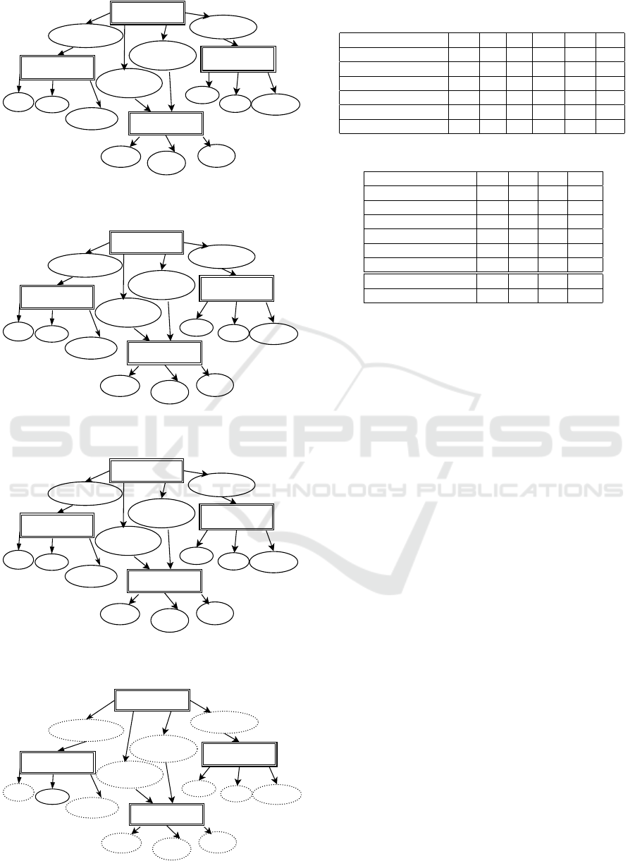
second test case is a failed one. For this test input, the
weights of each exercised dependency edge is multi-
plied by the factor w
f ail
. Figure 6 shows the modified
weights of the dependency edges after execution of
second test case. Figure 7 shows the resultant weights
of the dependency edges after all the seven test cases
are executed in which 5 test cases are pass and 2 are
failed. Figure 8 shows the normalized weights of the
dependency edges.
Figure 9 shows the weights of each function at
their function entry node (FEN). It is calculated by
taking the average weights of all the dependency
edges entering and leaving the node using Equation
6. Further, the function nodes are arranged based
upon their suspiciousness scores. It is observed that
the probability of the bug containment of the func-
tions is as: sub(a,b) > print(a,b,c) > main() >
add(a,b) It implies that the probability of presence
A Function Dependency based Approach for Fault Localization with D*
277
entry: main
entry: add
entry: print
entry: sub
call: add(a, b)
call:
print(a, b, c)
call:
print(a, b, c)
call: sub(a, b)
a=a_in
b=b_in
c_out=a+b
a=a_in
b=b_in c_out=a*b
a=a_in
b=b_in
c=c_in
1/1.5 3/0.5
5/1.5
7/0.5
9/1.5
16/0.5
17/0.5
10/1.5
11/1.5
12/.75
13/.75
14/.75
15/0.5
2/1.5
4/0.5
6/1.5
8/0.5
Figure 6: Modified weights of dependency edges after exe-
cution of the second test case.
entry: main
entry: add
entry: print
entry: sub
call: add(a, b)
call:
print(a, b, c)
call:
print(a, b, c)
call: sub(a, b)
a=a_in
b=b_in
c_out=a+b
a=a_in
b=b_in c_out=a*b
a=a_in
b=b_in
c=c_in
1/7.59
3/0.25
5/7.59
7/0.25
9/7.59
16/0.25
17/0.25
10/7.59
11/7.59
12/1.89
13/1.89
14/1.89
15/0.25
2/7.59
4/0.25
6/7.59
8/0.25
Figure 7: Modified weights of dependency edges after exe-
cution of seven test cases (5-Pass and 2-Fail).
entry: main
entry: add
entry: print
entry: sub
call: add(a, b)
call:
print(a, b, c)
call:
print(a, b, c)
call: sub(a, b)
a=a_in
b=b_in
c_out=a+b
a=a_in
b=b_in c_out=a*b
a=a_in
b=b_in
c=c_in
1/1
3/0.03
5/1
7/0.03
9/1
16/0.03
17/0.03
10/1
11/1
12/0.24
13/0.24
14/0.24
15/0.03
2/1
4/0.03
6/1
8/0.03
Figure 8: Normalize edge weights (by considering the high-
est weight as 7.59).
entry: main
entry: add
entry: print
entry: sub
call: add(a, b)
call:
print(a, b, c)
call:
print(a, b, c)
call: sub(a, b)
a=a_in
b=b_in
c_out=a+b
a=a_in
b=b_in c_out=a*b
a=a_in
b=b_in
c=c_in
0.515
0.03
1
0.35
Figure 9: Suspicious score of function at FEN by averaging.
Table 1: Values of various static metrics of functions present
in Figure 3.
Metrics print add sub main Max Min
Executable code line 1 2 2 10 10 1
Cyclomatic Complexity 1 1 1 2 2 1
No. of variables 3 2 2 3 3 2
Function Parameter 3 2 2 2 3 2
Max Nesting 0 0 0 1 1 0
Count Path 0 0 0 1 1 1
Table 2: Comprehensibility score of functions in Figure 3.
Metrics print add sub main
Executable code line 0 0.11 0.11 1
Cyclomatic Complexity 0 0 0 1
Number of variables 1 0 0 1
Function Parameter 1 0.66 0.66 0
Max Nesting 0 0 0 1
Count Path 0 0 0 1
Sum 2 0.77 0.77 5
Comprehensibility Score 0.23 0.09 0.09 0.585
of fault in sub() function is highest. Also, the fault
present in the sub() function. The statements of
sub(a,b) function is ranked according to a SBFL
technique.
Table 1 shows the values of different com-
plexity metrics for every function in the program.
These values were obtained through a static analy-
sis tool Understand-C(SCI-Tools, 2010). The last
two columns represent the highest and lowest value
for each metric, respectively. In Table 2, first six
rows represent the normalized value for every metric
through min-max normalization. Row 7 shows the ad-
dition of normalized values of complexity metrics for
each function. Row 8 presents the comprehensibility
score for each function computed using Equation 8.
4 EXPERIMENTAL STUDIES
We first discuss the setup used for experimental eval-
uation. Further, we present the subject programs and
estimation of heuristic parameters for the proposed
FDBD
∗
technique. Subsequently, we analyze the ob-
tained results.
4.1 Setup
We developed a prototype tool for our FL technique
and named it as FDBD
∗
tool. It was developed on
64-bit ubuntu 16.04 machine with 3.8 GB RAM. The
input is requested to be in ANSI-C format. Python
is used as a scripting language for developing all the
modules. The open-source tools used are Gcov (Gcov,
2005), MILU (Milu, 2008), and Understand-C (SCI-
Tools, 2010). We have used Gcov (Gcov, 2005) for
ICSOFT 2020 - 15th International Conference on Software Technologies
278
collecting test case execution results and coverage in-
formation. For creating mutants, MILU (Milu, 2008)
was used. Understand-for-C (SCI-Tools, 2010), a
static analysis tool, was used to measure various func-
tion complexity metrics.
4.2 Subject Programs
To evaluate the performance of FDBD
∗
, we used
the Siemens suite (SIR, 2005). It is considered as
a benchmark for comparing different FL techniques
(Jones et al., 2001; Wong et al., 2013; Dutta et al.,
2019). Table 3 presents the characteristics of all the
seven subjects present in the suite. The table con-
tains program name, total faulty versions, lines of
code (LOC), functions, executable LOC, and test suite
size for the respective programs in Columns 2, 3, 4,
5, and 6, respectively. Programs Print Tokens2 and
Print Tokens are used as a token identifier in the com-
piler. Schedule2 and Schedule are priority schedulers.
Replace, Tot info, and Tcas are used for text replace-
ment, information measurement, and traffic collision
avoidance system respectively.
Table 3: Program characteristics.
Program No. of LOC No. of No. of No. of
Name Faulty Func. Exec. Test
Versions LOC Cases
Print Tokens 7 565 18 195 4130
Print Tokens2 10 510 19 200 4115
Replace 32 521 20 244 5542
Tot info 23 406 7 122 1052
Tcas 41 173 9 65 1608
Schedule 9 412 18 152 2650
Schedule2 10 307 16 128 2710
4.3 Estimation of Heuristic Parameters
Potential values for heuristic parameters w
f ail
and
w
pass
for dependency scoring method (HWN) and
w
f ail
for another dependency scoring scheme (DSN)
are determined experimentally. For HWN scoring
scheme, we experimented with the values of w
pass
and w
f ail
within the range of [1.01 to 2.0] and [0.01
to 0.90] respectively with an interval of 0.01. Simi-
larly, for the DSN scoring scheme, we experimented
with changing the value of w
f ail
in the range of [0.01
to 0.90] and the same interval of 0.01. We observed
from the experimental results that HWN prioritize the
functions most effectively with the values of w
pass
and
w
f ail
in range of [1.01 to 1.50] and [0.01, 0.20] re-
spectively. Similarly, DSN performs best when the
value of w
f ail
lies in the range of [0.50, 0.90].
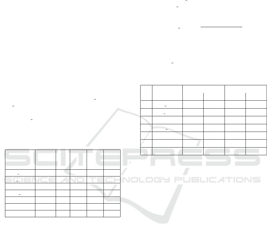
4.4 Evaluation Metric
To determine the effectiveness of our FDBD
∗
method,
we used the EXAM score metric (Renieres and Reiss,
2003). EXAM score for a program P is calculated
using Equation 9.
EXAM score =
|V
examined
| ∗ 100%
|V |
(9)
where, set V contains all the statements of program
P and set V
examined
consists of the statements exam-
ined during the bug localization. A technique with
lower EXAM Score is more effective in localizing the
faults.
Table 4: Function prioritization result.
S. Program HWN DSN
No. Name 1/3
rd
2/3
rd
1/3
rd
2/3
rd
1 Print Tokens 100.00% 100.00% 100.00% 100.00%
2 Print Tokens2 100.00% 100.00% 100.00% 100.00%
3 Replace 81.48% 100.00% 88.88% 100.00%
4 Tot Info 84.21% 100.00% 89.47% 100.00%
5 Tcas 81.08% 100.00% 91.89% 100.00%
6 Schdeule 100.00% 100.00% 100.00% 100.00%
7 Schdeule2 87.50% 100.00% 62.50% 100.00%
4.5 Results
This section discusses the result obtained for single-
fault localization.
4.5.1 Function Prioritization Result
Table 4 presents the function prioritization results
using our two reported dependency edge scoring
schemes: HWN and DSN for the Function Depen-
dency Graph. The table shows the percentage of ver-
sions for which the buggy function is ranked within
the top 1/3
rd
or 2/3
rd
of the prioritized functions
list. The obtained results for HWN and DSN scor-
ing schemes are shown in Columns 3, 4, and 5, 6,
respectively. It can be observed that for all the buggy
programs, the incorrect statement is present within the
top 2/3
rd
of the ranked functions. The HWN and DSN
schemes are effectively localized the faulty function
in the top 1/3
rd
of the prioritized functions list for an
average, 90.61% and 90.39% of buggy program ver-
sions.
4.5.2 Statement Localization Result
In this section, we compare the effectiveness of our
proposed FDBD
∗
approach with an established SBFL
A Function Dependency based Approach for Fault Localization with D*
279
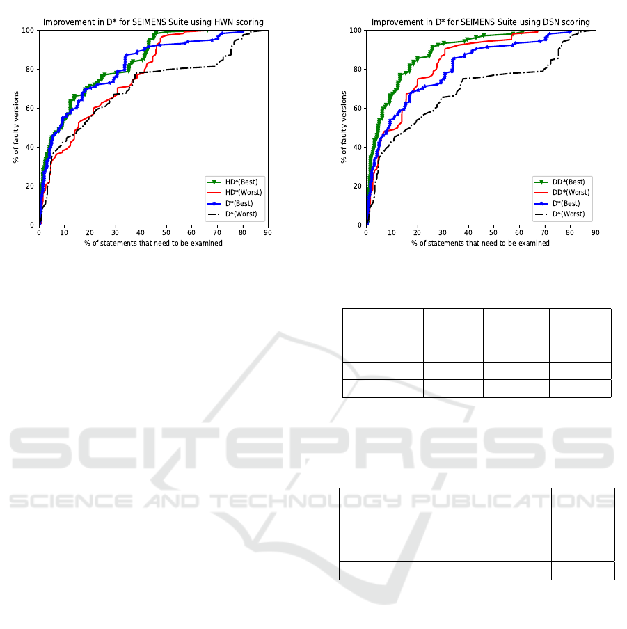
Figure 10: Effectiveness comparison of HD
∗
against D
∗
.
technique: DStar (Wong et al., 2013). SBFL tech-
niques assign two different types of effectiveness: the
best and the worst. For more details please refer
(Jones et al., 2001; Wong et al., 2016). Proposed
two different scoring techniques are combined with
D
∗
and referred to as DD
∗
and HD
∗
for DSN and
HWN scoring, respectively.
Figure 10 presents the effectiveness comparison
of HD
∗
against D
∗
using the Siemens suite. In the
line graphs, the x-axis and y-axis show the percent-
age of executable statements analyzed and the per-
centage of faulty program versions localized, respec-
tively. HD
∗
(Best) localizes bugs in 24.10% faulty ver-
sions by analyzing less than 1% of program code. On
the other hand, D
∗
(Best) localizes faults in 16.96%
of faulty versions only by checking the same percent-
age of program code. Likewise, HD
∗
(Worst) localizes
bugs in 42.85% of faulty programs by examining 5%
of program code whereas D
∗
(Worst) determine bugs
in 36.60% of faulty versions with the same percentage
of code examination. An interesting, as well as im-
portant observation, is that for many of the x values,
HD
∗
(Worst) is also performing better than D
∗
(Best).
There is an improvement of 32.31% in the worst-
case effectiveness of D
∗
by adding the FDG(HWN)
scheme, and this change is significant. A careful com-
parison shows that (i) HD
∗
(Best) is more adequate as
compared to D
∗
(Best) (ii) HD
∗
(Worst) is more ade-
quate than both D
∗
(Worst) and D
∗
(Best) with many
exam score points when all the faulty versions are
considered.
Table 5 presents the pairwise comparison between
the effectiveness of HD
∗
with D
∗
from three differ-
ent perspectives. It can be observed from the ta-
ble that HD
∗
(Best) is more effective than D
∗
(Best) in
58.03% of faulty program versions, equally effective
in 33.03% faulty versions and less effective in 8.92%
Figure 11: Effectiveness comparison of DD
∗
against D
∗
.
Table 5: Pairwise comparison between HD
∗
and D
∗
.
HD
∗
(Best) HD
∗
(Worst) HD
∗
(Worst)
vs D
∗
(Best) vs D
∗
(Worst) vs D
∗
(Best)
More effective 58.03% 62.50% 33.92%
Equally effective 33.03% 27.67% 12.50%
Less effective 8.92% 9.825% 53.57%
of versions. Similarly, HD
∗
Worst is either equal or
more effective as D
∗
(Worst) for 90.17% of faulty ver-
sions and least effective for only 9.73% of versions.
Table 6: Pairwise comparison between DD
∗
and D
∗
.
DD
∗
(Best) DD
∗
(Worst) DD
∗
(Worst)
vs D
∗
(Best) vs D
∗
(Worst) vs D
∗
(Best)
More effective 63.39% 68.75% 34.82%
Equally effective 31.25% 27.67% 16.07%
Less effective 5.35% 3.57% 49.10%
Figure 11 shows the effectiveness comparison of
DD
∗
with D
∗
over the Siemens suite. It can be ob-
served from the figure that DD
∗
(Best) is more effec-
tive than D
∗
(Best), DD
∗
(Worst) localizes bugs by ex-
amining less code than both D
∗
(Best) and D
∗
(Worst)
in many faulty programs. D
∗
(worst) requires to ex-
amine the complete program to localize the faults for
some programs. Whereas, DD
∗
(Worst) examines at-
most 67.18% of program code to localize faults in any
of the considered set of programs versions.
Table 6 presents a pairwise effectiveness compar-
ison between DD
∗
and D
∗
techniques. It can be ob-
served from the table that DD
∗
(Best) is at least as ef-
fective or more effective than D
∗
(Best) for 94.64%
of faulty programs. Only for the 5.35% of sub-
ject programs, DD
∗
(Best) performs less effectively
than D
∗
(Best). Similarly, only for 3.57% of versions
DD
∗
(Worst) is performing less code examination than
ICSOFT 2020 - 15th International Conference on Software Technologies
280

D
∗
(Worst). Also, DD
∗
(Worst) is at least as effective
as D
∗
(Best) in 50.89% of faulty versions. On aver-
age, our proposed DD
∗
performs 43.65%, and HD
∗
performs 38.88% more effectively than existing D
∗
.
5 MULTIPLE FAULTS
Till now, we have discussed the localization in single
fault programs. But, usually, a program contains more
than one fault. We discuss an extension of FDBD
∗
to
localize programs with more than one bug. It is a two-
step procedure. In the first step, we cluster the failed
test cases into fault-focusing clusters. Such that all
the tests present in a cluster are failed on account of
the same fault. Many techniques are available in the
literature to create fault-focused clusters (Jones et al.,
2007; Cellier et al., 2011). In the second step, each of
the failed test cases is merged with all the successful
test cases for localizing the targeted fault. We have
used the same approach as described in (Jones et al.,
2007) to generate the clusters of failed test cases. The
only difference is that instead of using SBFL tech-
niques (Tarantula or D
∗
) scores on all the statements,
we use our proposed method of selective function’s
statements scores to generate the fault focused clus-
ters. This way, we have extended our FDBD
∗
tech-
nique for localizing programs with multiple-faults.
We have injected two to four faults in different
programs. For comparison with existing approaches,
we have created fault focused clusters with their re-
spective scoring techniques. We have debugged the
program faults in parallel and reported the cumula-
tive EXAM score to localize all the bugs in that pro-
gram. Table 7 shows the comparison of the EXAM
score required by D
∗
, HD
∗
, and DD
∗
fault local-
ization techniques. Column 2 of the table is in
the format of ‘PName VNum’. Here PName de-
notes the program name, and VNum shows the cre-
ated faulty version number. Column 3 shows the to-
tal faults injected in the respective program version.
Columns 4-9 present the best and worst-case EXAM
scores of different techniques. On average, the ef-
fectiveness of HD
∗
(Best) is 4.31%, and HD
∗
(Worst)
is 2.90% better than D
∗
(Best) and D
∗
(Worst) respec-
tively. DD
∗
(Best) is 7.26% more competent than
D
∗
(Best), and DD
∗
(Worst) is 4.88% more effective
than D
∗
(Worst).
6 THREATS TO VALIDITY
We discuss the threats to the validity of our proposed
approach and obtained results:
1. The effectiveness of FDBD
∗
for FL relies on both
the number of pass and failed test inputs. If all
the test inputs are either completely pass or failed,
then, our approach may not localize the bug cor-
rectly.
2. In the paper, we experimented over a limited set of
programs. It is possible that our approach might
not work for specific types of programs. However,
to mitigate this risk, we have considered programs
with different functionality, size, faulty versions,
test inputs used, etc.
3. We have adopted EXAM
Score metric to check
the performance of our FDBD
∗
approach. But,
EXAM Score does not quantify the amount of
time spend by a developer to analyze a single
statement. So, we can not estimate the total
amount of effort spends by a developer to local-
ize the bugs.
4. The behavior of the program analyzer and test
case executor varies in different platforms (OS/
compiler). To mitigate this threat, we re-
implemented the existing FL technique and pro-
posed approach in the same machine.
7 COMPARISON WITH
RELATED WORK
Cleve et al. (Cleve and Zeller, 2005) reported a state-
model based FL technique and named it as cause tran-
sition. They identified the program points where the
root cause of failure is transferred from one variable
to the other variable. Cause transition is an exten-
sion of authors’ earlier work called delta debugging
(Zeller and Hildebrandt, 2002). Jones et al. (Jones
et al., 2001) showed that the FL technique Tarantula
is more effective than set union, set intersection, and
cause-transition approaches in terms of code exami-
nation. Based on our experimental results, it is ob-
served that our proposed FDBD
∗
approach is more
effective than Tarantula.
Renieris et al. (Renieres and Reiss, 2003) pro-
posed the nearest-neighbor approach for FL. They tar-
geted to find the most similar trace generated from the
successful test cases with a failed test case trace. Fur-
ther, they applied a set difference to eliminate the ir-
relevant statements from the failed test case trace and
returns a list of suspicious statements. The effective-
ness of their approach is completely dependent on the
used test suite. Also, in some cases, it returns a null
set of suspected statements. Whereas, FDBD
∗
uses
the test suite first to prioritize the function and then,
localized the bug at the statement level.
A Function Dependency based Approach for Fault Localization with D*
281
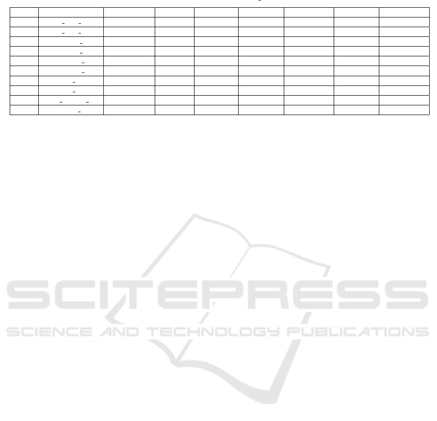
Table 7: Comparison of D
∗
with HD
∗
and DD
∗
based on the Exam Score metric for multiple fault localization.
S.No. Program No. of faults D
∗
(Best) D
∗
(Worst) HD
∗
(Best) HD
∗
(Worst) DD
∗
(Best) DD
∗
(Worst)
1 Tot Info V1 2 36.88% 45.90% 34.42% 43.44% 31.14% 40.16%
2 Tot Info V2 4 52.45% 68.85% 49.18% 65.57% 49.18% 65.57%
3 Schedule V1 3 35.52% 43.42% 28.94% 36.84% 28.94% 36.84%
4 Schedule V2 3 21.71% 35.52% 16.44% 30.26% 15.13% 28.94%
5 Schedule2 V1 4 37.50% 49.21% 45.31% 57.03% 43.75% 55.46%
6 Schedule2 V2 3 28.12% 46.87% 26.56% 45.31% 26.56% 45.31%
7 Tcas V1 3 55.38% 92.30% 52.30% 89.23% 52.30% 89.23%
8 Tcas V2 4 43.07% 89.23% 43.07% 89.23% 43.07% 89.23%
9 Print Tokens V1 2 22.56% 29.74% 24.61% 31.79% 23.58% 30.76%
10 Replace V2 4 49.18% 65.57% 45.08% 61.47% 40.98% 57.37%
In the literature, various slicing based FL tech-
niques are reported (Weiser, 1984; Agrawal and Hor-
gan, 1990). Slicing focused techniques return a list
of suspicious instructions, but these techniques do not
assign ranks to the instructions. Also, it is possible
that a slice may contain all the program instructions,
and this nullifies the performance of slicing. On the
other hand, our FDBD
∗
approach returns a ranked
list of statements present in the most suspicious func-
tions.
Wong et al. (Wong and Qi, 2009) was the first
to introduce neural networks (NN) for FL. Wong et
al. (Wong et al., 2010) also used RBF (radial basis
function) NN for the same. Dutta et al. (Dutta et al.,
2019) reported a hierarchical approach for FL using
deep neural networks (DNN). They have used DNNs
for both function and statement prioritization. NNs
easily map complex functions with the help of the
training set. However, NNs require a large amount
of time for parameter estimation and model training.
Whereas, the time required in each step of the pro-
posed FDBD
∗
is reasonable and deterministic. Hence,
our proposed approach will work efficiently for large-
size programs.
8 CONCLUSION
We have presented a hierarchical FL technique using
Weighted Function Dependency Graph (WFDG) and
existing SBFL technique D
∗
. The WFDG models the
function dependency information, and the weights as-
signed in the dependency edges indicate the relevance
of an edge in propagating a fault. With the help of
the weighted dependency edges, the functions are pri-
oritized. To differentiate between the functions with
equal suspiciousness value, we have incorporated the
information computed using static analysis. From our
experimental evaluation, it is observed that the pro-
posed FDBD
∗
technique is, on average, 41.27% more
effective than the existing SBFL technique D
∗
.
We extend our technique to handle object-oriented
programs. We also intend to investigate learning-
oriented methods to estimate the heuristic parameters.
REFERENCES
Abreu, R., Zoeteweij, P., and Van Gemund, A. J. (2009).
Localizing software faults simultaneously. In 2009
Ninth International Conference on Quality Software,
pages 367–376. IEEE.
Agrawal, H. and Horgan, J. R. (1990). Dynamic program
slicing. ACM SIGPlan Notices, 25(6):246–256.
Agrawal, H., Horgan, J. R., London, S., and Wong, W. E.
(1995). Fault localization using execution slices and
dataflow tests. In Proceedings of Sixth International
Symposium on Software Reliability Engineering. IS-
SRE’95, pages 143–151. IEEE.
Ardimento, P., Bernardi, M. L., Cimitile, M., and Ruvo,
G. D. (2019). Reusing bugged source code to support
novice programmers in debugging tasks. ACM Trans-
actions on Computing Education (TOCE), 20(1):1–
24.
Ascari, L. C., Araki, L. Y., Pozo, A. R., and Vergilio, S. R.
(2009). Exploring machine learning techniques for
fault localization. In 2009 10th Latin American Test
Workshop, pages 1–6. IEEE.
Cellier, P., Ducass
´
e, M., Ferr
´
e, S., and Ridoux, O. (2011).
Multiple fault localization with data mining. In SEKE,
pages 238–243.
Choi, S.-S., Cha, S.-H., and Tappert, C. C. (2010). A survey
of binary similarity and distance measures. Journal of
Systemics, Cybernetics and Informatics, 8(1):43–48.
Cleve, H. and Zeller, A. (2005). Locating causes of program
failures. In Proceedings. 27th International Con-
ference on Software Engineering, 2005. ICSE 2005.,
pages 342–351. IEEE.
Deng, F. and Jones, J. A. (2012). Weighted system depen-
dence graph. In 2012 IEEE Fifth International Con-
ference on Software Testing, Verification and Valida-
tion, pages 380–389. IEEE.
Dutta, A., Jain, R., Gupta, S., and Mall, R. (2019). Fault
localization using a weighted function dependency
graph. In 2019 International Conference on Quality,
Reliability, Risk, Maintenance, and Safety Engineer-
ing (QR2MSE), pages 839–846. IEEE.
ICSOFT 2020 - 15th International Conference on Software Technologies
282

Feng, M. and Gupta, R. (2010). Learning universal prob-
abilistic models for fault localization. In Proceed-
ings of the 9th ACM SIGPLAN-SIGSOFT workshop
on Program analysis for software tools and engineer-
ing, pages 81–88.
Gcov (2005). http://ltp.sourceforge.net/coverage/gcov.php.
Jones, J. A., Bowring, J. F., and Harrold, M. J. (2007). De-
bugging in parallel. In Proceedings of the 2007 inter-
national symposium on Software testing and analysis,
pages 16–26.
Jones, J. A. and Harrold, M. J. (2005). Empirical evalua-
tion of the tarantula automatic fault-localization tech-
nique. In Proceedings of the 20th IEEE/ACM inter-
national Conference on Automated software engineer-
ing, pages 273–282.
Jones, J. A., Harrold, M. J., and Stasko, J. T. (2001). Vi-
sualization for fault localization. In in Proceedings of
ICSE 2001 Workshop on Software Visualization. Cite-
seer.
Korel, B. (1988). Pelas-program error-locating assistant
system. IEEE Transactions on Software Engineering,
14(9):1253–1260.
Liu, C., Yan, X., Fei, L., Han, J., and Midkiff, S. P.
(2005). Sober: statistical model-based bug localiza-
tion. ACM SIGSOFT Software Engineering Notes,
30(5):286–295.
Mall, R. (2018). Fundamentals of software engineering.
PHI Learning Pvt. Ltd.
McCabe, T. J. (1976). A complexity measure. IEEE Trans-
actions on software Engineering, (4):308–320.
Miara, R. J., Musselman, J. A., Navarro, J. A., and Shnei-
derman, B. (1983). Program indentation and compre-
hensibility. Communications of the ACM, 26(11):861–
867.
Milu (2008). https://github.com/yuejia/milu.
Mund G. B., Goswami D, M. R. (2007). Program Slicing:
The compiler design handbook. CRC Press.
Renieres, M. and Reiss, S. P. (2003). Fault localization
with nearest neighbor queries. In 18th IEEE Interna-
tional Conference on Automated Software Engineer-
ing, 2003. Proceedings., pages 30–39. IEEE.
SCI-Tools (2010). https://scitools.com/.
SIR (2005). http://sir.unl.edu/portal/index.php.
Spinellis, D. (2018). Modern debugging: the art of finding
a needle in a haystack. Communications of the ACM,
61(11):124–134.
Thaller, H., Linsbauer, L., Egyed, A., and Fischer, S.
(2020). Towards fault localization via probabilis-
tic software modeling. In 2020 IEEE Workshop on
Validation, Analysis and Evolution of Software Tests
(VST), pages 24–27. IEEE.
Weiser, M. (1984). Program slicing. IEEE Transactions on
software engineering, (4):352–357.
Wong, W. E., Debroy, V., and Choi, B. (2010). A fam-
ily of code coverage-based heuristics for effective
fault localization. Journal of Systems and Software,
83(2):188–208.
Wong, W. E., Debroy, V., Gao, R., and Li, Y. (2013). The
dstar method for effective software fault localization.
IEEE Transactions on Reliability, 63(1):290–308.
Wong, W. E., Gao, R., Li, Y., Abreu, R., and Wotawa, F.
(2016). A survey on software fault localization. IEEE
Transactions on Software Engineering, 42(8):707–
740.
Wong, W. E. and Qi, Y. (2009). Bp neural network-based
effective fault localization. International Journal of
Software Engineering and Knowledge Engineering,
19(04):573–597.
Yu, X., Liu, J., Yang, Z., and Liu, X. (2017). The bayesian
network based program dependence graph and its ap-
plication to fault localization. Journal of Systems and
Software, 134:44–53.
Zeller, A. and Hildebrandt, R. (2002). Simplifying and iso-
lating failure-inducing input. IEEE Transactions on
Software Engineering, 28(2):183–200.
A Function Dependency based Approach for Fault Localization with D*
283
