New Traffic Congestion Analysis Method in Developing
Countries (India)
Tsutomu Tsuboi
*
Global Business Development, Nagoya Electric Works Co., Ltd., 29-1 Mentoku Shinoda, Ama Aichi, Japan
Keywords: Traffic Flow, Traffic Density, Traffic Congestion.
Abstract: This manuscript describes introducing new traffic congestion analysis for developing country in India. In
generally, it is challenge to show how traffic congestion occurs, especially in developing countries such as in
India because its traffic is consisted of various kinds of transportation like two wheelers, three wheelers, and
sometimes animals on the roads. There is a chance to collect real traffic flow data in Ahmedabad of Gujarat
states of India since October 2014. The traffic monitoring system there consist of 14 traffic monitoring
cameras and the system is capable to monitor traffic density, traffic volume, average vehicle speed, and
occupancy at the each location. In this manuscript, there are three types of traffic congestion analysis. One is
based on its observation traffic flow, in which it compares daily traffic volume and its average vehicle speed.
The second one is based on the judgement of occupancy parameter, which uses as one of traffic congestion
parameter in general. The third one is based on estimation from “social loss” calculation which comes from
the traffic flow theory but is challenge to analyse in the developing countries. The social loss calculation is
proven in the traffic theory but it is difficult to define the traffic demand curve, the social cost curve, and the
traffic supply curve. Author shows how to make the practical “social loss” calculation and its validation
compared with the actual traffic congestion condition.
1 INTRODUCTION
According to rapid economic growth in developing
countries such as India and China, it becomes big
issues of negative impact by transportations. An
economic growth requires transporting not only
people but also commercial goods and material
exporting to other countries and or importing as well.
In general, developing countries don’t spend enough
infrastructure improvement budget compared
growing economics. Therefore they have traffic
congestion, more accidents, environment problems
like air pollution, and untuneful energy consumption.
It is able to say that those issues are occurred by poor
infrastructure development and growth of traffic. And
it is not easy to manage proper traffic condition under
this situation, particularly to analyse traffic condition
of developing countries. There are not so many study
of traffic flow analysis for the developing counters.
The traffic flow analysis is introduced by
Goutham.M, Chanda.B in “ Introduction to the
selection of corridor and requirement,
*
https://www.nagoya-denki.co.jp/en/
implementation of IHVS (Intelligent Vehicle
Highway System) In Hyderabad. This research took
only few days data collection. And the other one is
headway parameter analysis in India by Salim.A,
Vanajakshi.L, Subramanian.C but its data is based on
only four days measurement.
Author have a chance to manage intercity traffic
by ITS or Intelligent Transport Systems business in
one of major city of India 2014. The city is
Ahmedabad which is located in Gujarat State of west
Side of India. The system of ITS (Intelligent
Transport System) has fourteen traffic monitoring
cameras and four traffic information display which is
called “VMS” or Variable Message Sign board.
Traffic condition such as traffic volume, traffic
density, gaps between vehicles are observed by the
system and traffic congestion level is provided
through VMS to drivers. Therefore motivation is to
analyse Indian traffic condition on the basis of one
month measurement in June 2015 from the ITS
system in Ahmedabad. The detail ITS system
Tsuboi, T.
New Traffic Congestion Analysis Method in Developing Countries (India).
DOI: 10.5220/0009766501450151
In Proceedings of the 6th International Conference on Vehicle Technology and Intelligent Transport Systems (VEHITS 2020), pages 145-151
ISBN: 978-989-758-419-0
Copyright
c
 2020 by SCITEPRESS – Science and Technology Publications, Lda. All rights reserved
145

configuration and location are described in the next
section.
2 TRAFFIC FLOW ANALYSIS
2.1 Measurement Field and Data
The ITS system in Ahmedabad consists of 14 CCTV
or traffic monitoring cameras and for VMSs in the
city. The Figure 1 shows the location of each CTV
and VMS in the city. In Figure 1, Cam#1 means
CCTV number 1 and Cam#1 has one CCTV with pole
on the street. The VMS#1 means VMS number 1 and
it also has CCTV with Traffic Sign board.
The traffic data is measured by the CCTV and
measures traffic flow data such as number of vehicles,
average vehicles speed, traffic density. In this paper,
it is used this traffic flow data in June 2015 one month
data by every minutes. The total traffic flow data for
each CCTV becomes more than 40,000 points and
author took 11 camera data through camera number 1
to 10 and VMS number. In this paper, we take eleven
CCTV data because VMS#1 and VMS#2 data are
missing during measurement by communication
network error.
Figure 1: Traffic monitoring camera location in
Ahmedabad city.
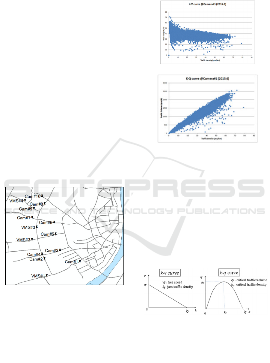
In terms of measurement data, Figure 2 shows two
typical traffic flow characteristics―traffic density (k)
to vehicle average speed (v) and traffic density (k) to
traffic volume (q) of Cam#1 in June 2015.
In terms of traffic measurement value, all these value
are generalized as one lane of each road for the
comparison of traffic condition level among the
different number of lanes roads. The two lanes of road
is at through Cam#1 to Cam#7 and through VMS#1
to VMS#4. The three lanes is at through Cam#8 to
(a) k - v curve at Camera #1.
(b) k - q curve at Camera #1.
Figure 2: Traffic Flow Characteristic of Cam#1.
Cam#10. Therefore the actual value of .traffic volume
and density are the described value times by each
number of lanes.
2.2 Traffic Flow Theory
In the traffic flow theory, there are typical
characteristics which are defined relationships traffic
density (k) and traffic volume (q) ―k – q curve― and
traffic density (k) and average vehicle speed (v)―k –
v curve― which are illustrated in Figure 3. In terms
of k – v curve, there are three major curves e.g.
Greenshields, Greenburg and Underwood. In this
paper, we use most typical Greenshields one.
(a) k – v curve (b) k- q curve
Figure 3: Traffic Flow Characteristic of Cam#1.
From the traffic flow theory, the k – v curve and k – q
curve are provided by equation (1) (2) (3) and (4).
𝑣=𝑣

1 
𝑘
𝑘


(1)
VEHITS 2020 - 6th International Conference on Vehicle Technology and Intelligent Transport Systems
146

𝑞=
𝑣

𝑘

𝑘
𝑘

2



𝑣

𝑘

4
(2)
𝑞

=
𝑣

𝑘

4
(3)
𝑘

=2𝑘

(4)
where v
f
is free vehicle speed, k
j
is jam traffic density,
q
c
is critical traffic volume, and k
c
is critical traffic
density.
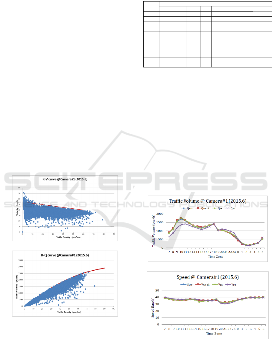
From Figure 2 (a) and (b), we see there is
boundary line in each curve and there is no data over
its boundary line. Therefore this boundary line means
each traffic flow characteristics. There are similar
kind of characteristics in all other CCTVs. From this
observation method, we have traffic flow parameters
fitting by equation (1) and (2). Figure 4 shows each
boundary line on both k–v curve and k–q curve. From
this observation method, the boundary line is able to
be drawn by using equation (1) and (2). Based on this
observation method, it is able to get traffic flow
parameters ―v
f
, kj, and qc― and curve equation (1),
(2). The summary of all CCTV data is shown in Table
1.
(a) k - v curve at Camera #1 with boundary edge line.
(b) k - q curve at Camera#1 with boundary edge line.
Figure 4: Traffic Flow Curve with boundary line.
Table 1: Summary of Traffic flow equation and parameters.
2.3 Traffic Congestion
In order to analyse the traffic congestion from
measurement data, there are several method.
 Observation from daily traffic flow
 Judgement from occupancy parameter
 Judgement by Social Loss calculation
From the next section, each analysis is described.
2.3.1 Observation from Traffic Flow
This observation is to define the traffic congestion by
comparing daily number of vehicle and average speed
for each hour. Figure 5 shows an example of Cam#1
traffic flow daily data and (a) shows time zone basis
number vehicle trend and (b) shows average vehicle
speed.
(a) Traffic volume of Camera#1.
(b) Traffic average speed of Camera#1.
Figure 5: Traffic Flow Time Zone basis Measurement.
v ｆ /k
j
k
c
q
c
v
c
Formula v
f
Cam#1 0.2479 110 3,000 27 -0.2479(
k
-110)^2+3000 54.545
Cam#2 0.1556 150 3,500 23 -0.1556
(
k
-150
)
^2+3500 46.667
Cam#3 0.2153 120 3,100 26 -0.2153(
k
-120)^2+3100 51.667
Cam#4 0.3200 100 3,200 32 -0.3200(
k
-100)^2+3200 64.000
Cam#5 0.3704 90 3,000 33 -0.3704(
k
-90)^2+3000 66.667
Cam#6 0.2367 130 4,000 31 -0.2367(
k
-130)^2+4000 61.538
Cam#7 0.2361 120 3,400 28 -0.2361(
k
-120)^2+3400 56.667
Cam#8 0.3200 100 3,200 32 -0.3200
(
k
-100
)
^2+3200 64.000
Cam#9 0.4898 70 2,400 34 -0.4898(
k
-70)^2+2400 68.571
Cam#10 0.3438 80 2,200 28 -0.3438(
k
-80)^2+2200 55.000
VMS#3 0.2361 120 3,400 28 -0.2361(
k
-120)^2+3400 56.667
Location
Data analysis
New Traffic Congestion Analysis Method in Developing Countries (India)
147

From Figure 5 (a), there are two peeks of number of
traffic volume in the morning from 9:00 to 11:00 and
the evening from 17:00 to 19:00. Form Figure 5 (b),
the average vehicle speed seems to be stable or not so
much drop at those two traffic peeks. The vehicle
speed in the evening peek is relatively lower than in
the morning peek. From this observation, there is no
traffic congestion at Cam#1 in June 2015.
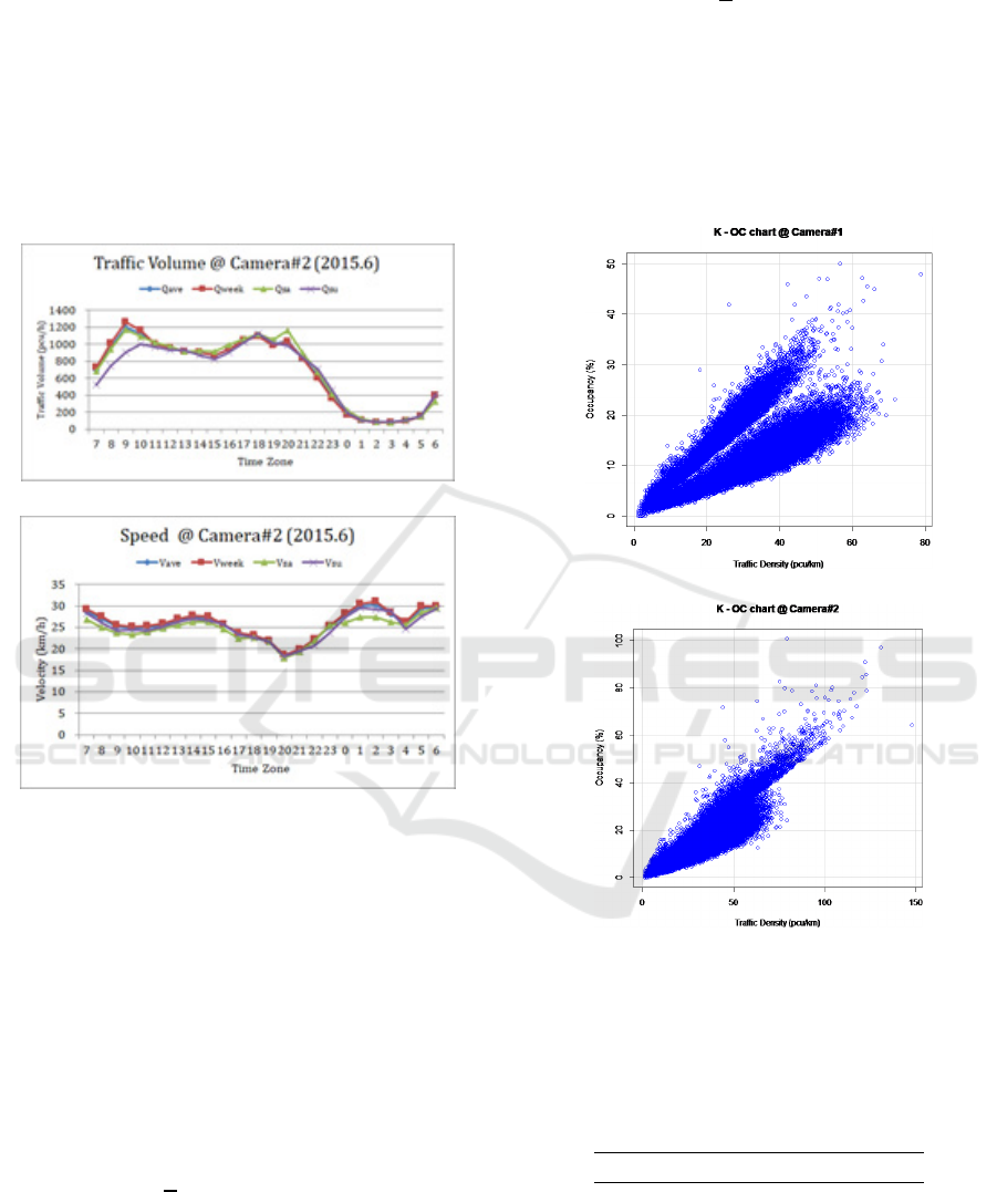
On the other hand, Figure 6 shows the case of Cam#2.
(a) Traffic volume of Camera#2.
(b) Traffic average speed of Camera#2.
Figure 6: Traffic Flow Time Zone basis Measurement.
From Figure 6 (a), there are two traffic number of
vehicle as same as Cam#1. But from Figure (b), there
is big speed drop in the evening, which means there
is traffic congestion.
2.3.2 Judgement from Occupancy
In this section, occupancy (OC) is introduced as one
of traffic flow parameter for traffic congestion
indication. From traffic flow theory, (OC) is defied
by equation (5).
𝑂𝐶=
1
𝑇
𝑡


× 100

%

(5)
where T is time of measurement, t
i
is detected time of
vehicle i.
When number of existing vehicle a certain section
is N, average length of vehicle is 𝑙
̅
, formula (6) is
given.
𝑂𝐶 =100
𝑞
𝑣
𝑙
̅
=100 𝑘𝑙
̅
(6)
Therefore occupancy (OC) is proportional to traffic
density (K) and traffic volume (q).From the one
month measurement data of Cam#1 and #2 in June
2015, traffic density (k) to occupancy (OC)
relationship are shown in Figure 7. According to
Figure 7, the relationship between (k) and (OC) is
proportional but the dispersion of data is seen.
(a) k-OC characteristics of Cam#1.
(b) k-OC characteristics of Cam#2.
Figure 7: Example of k-OC characteristics.
In order to identify time zone basis characteristics, six
time zone is introduced from T1 to T6 as shown in
Table 2.
Table 2: Time Zone Classification.
Zone Name Time Zone
T1 7:00 – 10:59
T2 11:00 - 14:59
T3 15:00 - 18:59
T4 19:00 - 22:59
T5 23:00 - 2:59
T6 3:00 - 6:59
VEHITS 2020 - 6th International Conference on Vehicle Technology and Intelligent Transport Systems
148

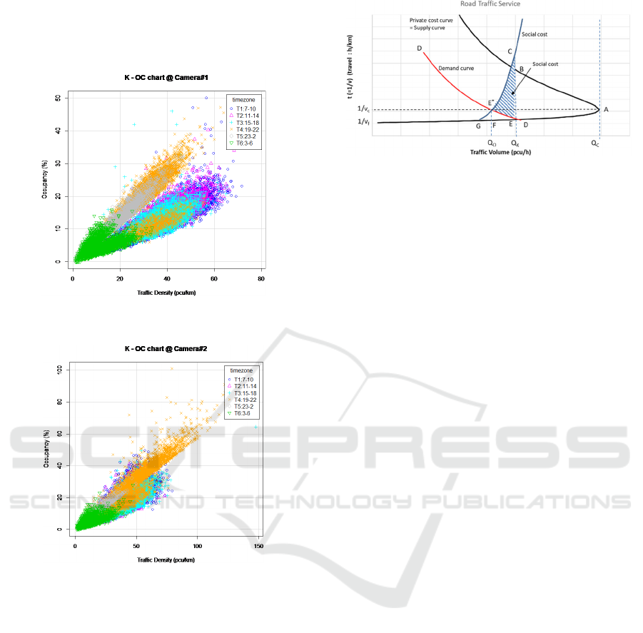
By using Time Zone in Table 2 for Figure 7, then
Figure 8 is obtained. From Figure 8, it is clear that T4
is most congested condition and the condition of (OC)
over 30% is congested.
(a) Time Zone based k – OC chart at Cam#1.
(b) Time Zone based k – OC chart at Cam#2.
Figure 8: Time Zone based of k-OC characteristics.
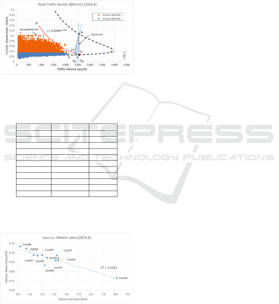
2.3.3 Judgement from Social Loss
Finally, Social Loss is introduced in this section.
According to the traffic flow theory, the Social Loss
caused by traffic congestion is defined the Traffic
Road Service Market Model. The theoretical Social
Loss is calculated by area CE*E in Figure 9.
In Figure 9, the supply curve line rises to the right
from travel time (1/v
f
) to (1/v
c
), which means private
cost curve for transportation. And when (v) becomes
small (travel time (t) becomes large), the value in
blanket becomes negative and the supply curve drops
to the right, which corresponds to private cost curve.
Figure 9: Traffic Road Service Market Model.
The point A is called hyper congestion condition
at critical traffic volume (q
c
) when traffic volume
becomes larger beyond point A, travel time takes
more because of traffic congestion. There are two
travel time (t) except point A. In case of travel time
longer at point B, there is travel service loss in terms
of transport efficiency because travel time takes more
than that of point E same which has equivalent traffic
volume. If traffic demand curve D-D is given, the
point E is cross point between demand curve D-D and
supply curve which provides balance condition
between traffic demand and supply condition. When
social cost curve is given, the point E* becomes
balance point between traffic demand and social cost.
Then area CE*E provides traffic service cost loss
caused by traffic congestion because infrastructure
should cover at the level of traffic volume (Q
x
) at the
point E and social cost rises at the point C where its
traffic volume (Q
x
) is same as that of at the point E.
Therefore area CE*E is defined as “Social Cost” by
traffic congestion.
In our previous work of traffic flow analysis in
CODATU November 2017, the critical vehicle speed
(v
c
) is 2/3 times of free speed (v
f
). Therefore Figure 8
shows the result of measurement plot of Camera#2.
In order to get the graph, we use the following
condition.
 Demand curve: it is set on the boundary
approximate line of all measurement plots
 Social cost: it is defined by linear line between
point E* and point B. The traffic volume at
point B is equal to that of point E. The point E
is cross point of supply curve and boundary
approximate line of measurement data.
On the basis of the above conditions, we define area
BE*E as social cost. This definition is not exactly
same as that of Figure 9 but it is enough to use this
parameter as equivalent of social cost because we
want to have relative comparison among
measurement result in Ahmedabad traffic with
common parameter—equivalent social cost.
According to the definition of point E*, it should be
New Traffic Congestion Analysis Method in Developing Countries (India)
149

cross point of supply curve at the travel time level
(=1/v
c
) at point A in Figure 9. But we already see the
threshold between congested traffic flow condition
and free flow condition is at threshold point of which
inverse of vehicle velocity equals to 1/(2v
f
/3).
Therefore point E* in Figure 10 is set at t = 1/ (2v
f
/3).
Under these conditions, social cost of each road is
obtained by area BE*E in Figure 10.
Figure 10: Traffic Road Service Market at Cam #2.
Table 3 shows the summary of Social Loss value of
each CCTV.
Table 3: Social cost and speed ratio comparison.
Location
v
ave
/
v
f
Social loss
Cam#1 0.66 3.3
Cam#2 0.57 8.1
Cam#3 0.66 3.1
Cam#4 0.69 3.2
Cam#5 0.69 2.0
Cam#6 0.63 2.2
Cam#7 0.69 1.3
Cam#8 0.73 0.2
Cam#9 0.69 1.6
Cam#10 0.67 2.4
VMS#3 0.72 0.7
The correlation between speed ratio and social
loss is shown in Figure 11 and calculated Social Loss
is able to be representative value of traffic congestion
(the decision factor R
2
=0.825).
Figure 11: Correlation between Social cost and Vehicle
ratio.
3 CONCLUSIONS
In this paper, author provides three types of traffic
congestion analysis by typical traffic flow
measurement observation, occupancy judgement, and
Social Loss calculation. From these analysis, we
know the total hourly number of vehicle of each road
is not always explained the traffic congestion. From
traffic flow measurement observation, the second
number of vehicle peek point in the evening is most
congested condition. From occupancy judgement, T4
(which means the time frame from 19:00 to 22:59) is
most congested time zone. This is the same as traffic
flow observation. In Social Loss calculation,
calculated Social Loss is able to define the one of
traffic congestion parameter.
This research continues to collect traffic flow data
in Ahmedabad and a whole year analysis brings us
more detail thought about Indian traffic congestion
analysis. After this research, we will find out the
traffic condition reason. The more traffic flow
parameter value comparison is required in future
work. Some future work introduction is described in
Appendix. It is also necessary to make spatial analysis
after collection all traffic flow data collection points.
ACKNOWLEDGEMENTS
This research is part of SATREPS program 2017 (ID:
JPMJSA1606)) between India and Japan.
REFERENCES
Goutham.M, Chanda.B, 2014 , Introduction to the selection
of corridor and requirement, implementation of IHVS
(Intelligent Vehicle Highway System) In Hyderabad,
International Journal of Modern Engineering Research,
Vol.4, Iss.7, pp.49-54
Salim.A, Vanajakshi.L, Subramanian.C, 2010, Estimation
of Average Space Headway under Heterogeneous
Traffic Conditions, International . of Recent Trends in
Engineering and Technology, Vol. 3, No. 5
Greenshields B.D., 1935, A Study of Traffic Capaci,
Proc.H.R.B., 14, pp.448-477
Greenberg, H. 1959, An analysis of traffic flow. Operation
Research, pp.79-85
Underwood, R. T. 1961, Speed, Volume, and Density
Relationship. Quality and Theory of Traffic Flow, Yale
Bur. Highway Traffic, New Haven, Connecticut,
pp.141-188
Tsuboi.T , Yoshikawa.N, : Traffic Flow Analysis in
Emerging Country (India), CODATU XVII, Nov.2017.
VEHITS 2020 - 6th International Conference on Vehicle Technology and Intelligent Transport Systems
150

Tsuboi.T, Oguri.K 2016, Journal of Society of Information
Processing Engineers, Vol. 57 No. 12, pp. 2819-2826
(in Japanese).
Matsuoka.Y, et al, 2013, Fluid Mechanics —Fundamentals
and Exercises—, Corona Publishing C. Book, pp.119-
121.
Kuroda.T, et al, 2008, Urban and Regional Economics,
Yuhikaku Book, pp. 265-268.
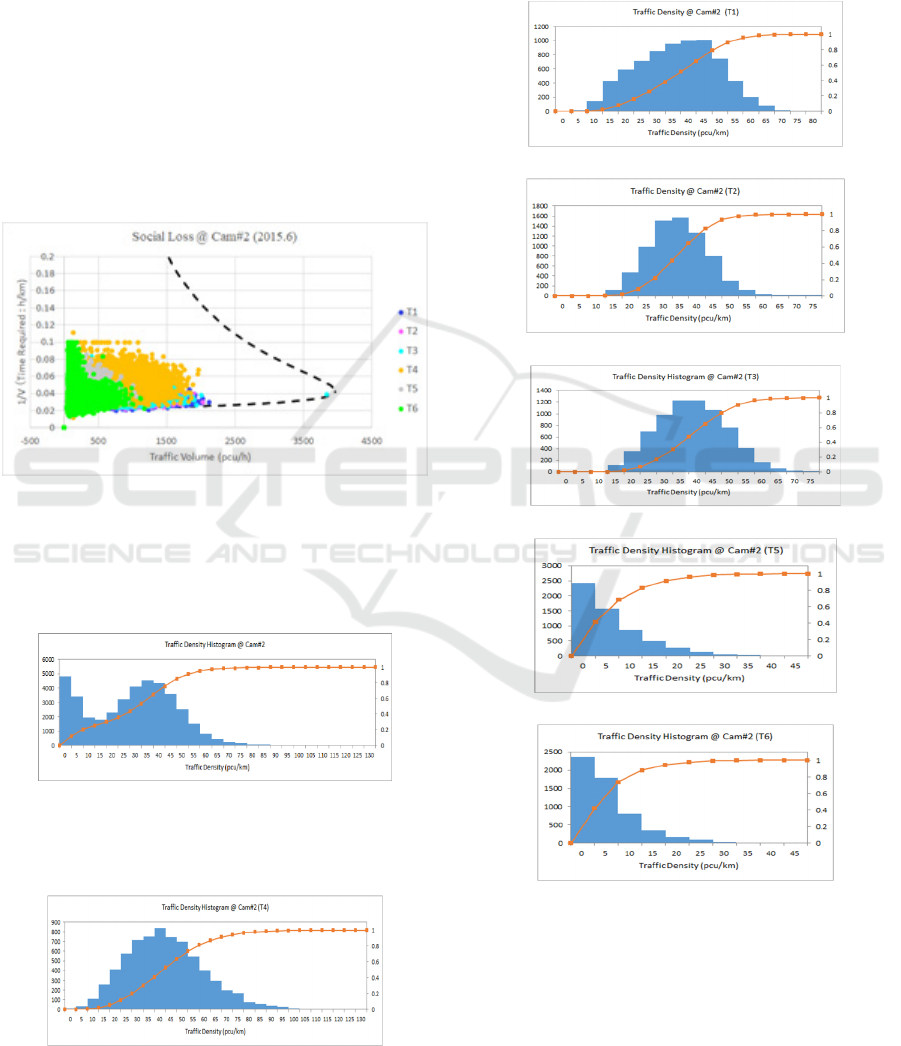
APPENDIX
In Social Loss research, the following Figure A shows
time zone basis characteristics. Form the Figure A, it
is clear that T4 time Zone is critical for traffic demand
curve.
Figure A: Time Zone basis Traffic Road Service Market at
Cam #2.
In case of traffic density histogram of Cam#2, there
are two peeks: one is low density point in T5 and T6,
the other is high density in T1 and T2 (Figure B).
Figure B: Traffic Density Histogram at Cam #2.
In terms of the traffic density in T4, Figure C shows
its histogram.
Figure C: Traffic Density Histogram in T4 at Cam #2.
From those two histograms of Figure B and C, the
traffic congestion condition courses under the
condition of traffic density which is from 20 to 60.
From Figure C, the traffic density histogram looks the
normal distribution. In Figure D, it shows other time
zone basis traffic density histograms as the reference.
(a) Traffic Density Histogram in T1 of Cam#2.
(b) Traffic Density Histogram in T2 of Cam#2.
(c) Traffic Density Histogram in T3 of Cam#2.
Figure D.
(e) Traffic Density Histogram in T6 of Cam#2.
Figure D: Traffic Density Histogram in each Time Zone.
Here is some notice about traffic flow values.
The value of the traffic density is generalized value
which is mentioned in section 2.1. Therefore the
number of lanes at Cam#2 is two lanes. So the real
traffic density here becomes two times.
New Traffic Congestion Analysis Method in Developing Countries (India)
151