
Data Mining Algorithms for Traffic Interruption Detection
Yashaswi Karnati, Dhruv Mahajan, Anand Rangarajan and Sanjay Ranka
Department of Computer and Information Science and Engineering, University of Florida, Gainesville, FL, U.S.A.
Keywords:
Incident Detection, Loop Detectors Systems, Traffic Interruptions, Semi-Supervised, Data Mining.
Abstract:
Detection of traffic interruptions (caused by vehicular breakdowns, road accidents etc.) is a critical aspect
of managing traffic on urban road networks. This work outlines a semi-supervised strategy to automatically
detect traffic interruptions occurring on arteries in urban road networks using high resolution data from widely
deployed fixed point sensors (inductive loop detectors). The techniques highlighted in this paper are tested on
data collected from detectors installed on more than 300 signalized intersections.
1 INTRODUCTION
Managing traffic incidents is one of the crucial ac-
tivities for any traffic management center. These in-
cidents are non-recurrent, may arise due to different
causes like traffic accidents, vehicle breakdowns, de-
bris etc. and cause congestion. It is worth noting that
not all accidents (e.g. a fender-bender) result in in-
terruptions. From a traffic management perspective,
it is more important to detect significant interruptions
rather than accidents. Further, this should be done
in real-time so that proactive actions can be used for
mitigation. Broadly, we define an interruption to be
any time period where the amount of traffic is sig-
nificantly lower than normal traffic for a significant
period of time. The focus of this study is in detect-
ing these events of interest from inductive loop detec-
tors installed at signalized intersections. While direct
and manual traffic management center (TMC) mon-
itoring has been adequate for previous years, many
TMCs have had limited operational use of automatic
incident detection techniques. This is due to these
techniques’ high rates of false alarms, complex cal-
ibration, and low detection rates (Williams and Guin,
2007). In fact, many automatic incident detection al-
gorithms perform poorly in the real world, compared
to simulated traffic environments (Parkany and Xie,
2005) (and please see Section 2 for more details).
Our goal in this paper is to use loop detector data
for detecting traffic interruptions. Loop detector data
are now widely available to traffic management per-
sonnel. Additionally, with new ATSPM based sys-
tems, such data is available at high frequency (10
Hz) and with low latency. Hence, the utilization of
this data for determining traffic interruptions can have
wide applicability and can be used in conjunction
with other systems based on human reporting or with
probe-based systems. Previous work using loop de-
tector data is generally limited to simulation or small
datasets (Section 2). In our work, we utilize 6 months
of data for 300 intersections to demonstrate the use-
fulness of our method. This dataset is roughly 700
GB in size. We believe that it is the first study that
uses fine grain (10Hz) ATSPM data for a large geo-
graphical region and over a long duration of time.
As mentioned, we seek to design algorithms to de-
tect traffic interruptions in a relatively unsupervised
fashion. We define traffic interruption as a signif-
icant, contextual and nonrecurring change observed
in a combination of the following parameters: the
amount of deviation of traffic volumes from predicted
volumes and the duration for which the actual traf-
fic volume deviated from the predicted volume. The
first step in this process is to analyze and pre-process
raw data gathered from fixed-point sensors or detec-
tors (Section 3). Once the data has been processed,
the next step in the pipeline is quantifying what an in-
terruption is and also labeling said traffic interruptions
(Section 4). The third step is to develop algorithms for
predicting the labeled interruptions (Section 5). If the
data is available in real-time with as low a latency as
practical, this considerably aids our effort. We list
three major contributions of our work:
1. Labeling data is a major challenge for big data ap-
plications since interruption ground truth is gen-
erally not available. We provide a rigorous defi-
nition and mechanism for automatically labeling
events of interest (EOI), i.e. large traffic reduc-
tions for long periods) from historical data.
106
Karnati, Y., Mahajan, D., Rangarajan, A. and Ranka, S.
Data Mining Algorithms for Traffic Interruption Detection.
DOI: 10.5220/0009422701060114
In Proceedings of the 6th International Conference on Vehicle Technology and Intelligent Transport Systems (VEHITS 2020), pages 106-114
ISBN: 978-989-758-419-0
Copyright
c
2020 by SCITEPRESS – Science and Technology Publications, Lda. All rights reserved

2. We develop a time-series based analysis system
for detecting if an event of interest has occurred.
This uses traffic information from recent time pe-
riods as well as historical data (from similar time
periods on previous days or weeks) to predict
if an event of interest—defined as a long traffic
interruption—has occurred. Whether or not an
EOI has occurred depends on a key parameter—
the duration of time after reduction in traffic at a
single detector. This has an impact on the over-
all accuracy (in terms of false positives and false
negatives). In particular, we find that waiting for
60 to 90 seconds after a significant reduction in
traffic is reasonable to determine EOIs with high
accuracy and low latency.
3. We perform a Spatio-temporal analysis of all
EOIs to determine if there are hotspots (i.e. in-
tersections with a large number of consistent
EOIs) and spatial relationships (two EOIs occur-
ring at neighboring intersections within a small
time frame). This analysis shows that most of the
EOIs are limited to around 10 (out of 300) inter-
sections and roughly 5% of all EOIs are spatially
correlated.
All of our methods are evaluated on six months of
data collected from Seminole County, Florida for
300+ intersections.
2 RELATED WORK
The existing literature pertaining to incident detection
can be broadly classified as follows:
1. Traditional systems which rely on inductive loops
and video cameras for vehicle detection.
2. Probe-based systems (GPS data from fleets of ve-
hicles like NavTech or HERE data).
3. Human reporting systems like calls to traffic man-
agement centers or the use of social media plat-
forms (like twitter).
There is also some work on using a combination
of multiple data sets. Most of the existing research in
automatic incident detection is focused on freeways
and or uses simulated data. The basic idea behind
these approaches is that if an incident occurs, there
would be a significant decrease in the occupancy at
the downstream detectors and increase in occupancy
at upstream detectors (Ahmed and Hawas, 2012), (Lin
and Daganzo, 1997), (Lee and Taylor, 1999). Urban
road networks with a high density of signalized in-
tersections behave differently from freeways due to
the influence of traffic signals, pedestrian crossings,
etc. Designing algorithms for incident detection on
arterial roads can hence be more challenging as com-
pared to doing the same for freeways. In (Jeong et al.,
2011; Teng and Qi., 2003; Jin et al., 2002; Lin and
Daganzo, 1997), incident detection models for free-
ways/highways are presented. Most of these methods
rely on detecting changes in the free-flowing state of
traffic and use thresholds for space-time detector oc-
cupancy driven by historical trends. Incidents are de-
tected by comparing current occupancy or speed value
with the derived thresholds.
There is an extensive body of research (Balke
et al., 1996; Mouskos et al., 1999; Yang et al., 2017;
Park and Haghani, 2016) on incident detection using
probe-based systems. The advantage of probe data
over fixed detector data is that probe data cover longer
sections of the road which can also be used to de-
tect secondary incidents (Yang et al., 2017; Park and
Haghani, 2016). But these algorithms highly depend
on the penetration rate of the probe car and confidence
level of the data. Also, algorithms based on human
reporting systems make use of sources like Twitter,
phone calls, Waze etc. These methods are highly de-
pendent on the availability of such data. This data is
generally sold by companies and can be expensive.
In (Gu et al., 2016), the authors presented methods
to mine tweet texts and extract information related to
incidents. The focus of our work is on using ground
sensors at intersections: this data is freely available
to transportation agencies and is routinely collected.
Also, our focus is on detecting traffic interruption
using sensor data (detector data) from road arteries.
Since the traffic patterns on arterials are significantly
different from highways, the problem is significantly
more challenging.
Existing research on incident detection on arteri-
als (Ahmed and Hawas, 2012; Lingras and Adamo,
1996) relies on simulated data (and accidents) or as-
sumes the availability of ground truth (either using
simulations or labeling). Due to this, many automatic
incident detection algorithms perform poorly in real-
world scenarios when compared to simulated environ-
ments (Parkany and Xie, 2005). Moreover, develop-
ing an incident data-set with start and end times can
be tedious and requires manual investigation by TMC
personnel. Taking into account the issues highlighted
above, this work focuses on detecting traffic interrup-
tions based on real, fixed point sensor data (detector
data) collected from signalized intersections and de-
tectors on urban road networks. In the next sec-
tion, we focus on the data processing needed for near-
realtime incident detection. Due to the real-world fo-
cus, we believe that the results presented in this paper
can be translated into practice.
Data Mining Algorithms for Traffic Interruption Detection
107

3 DATA PREPROCESSING
Traffic signal controller logs and the derived Au-
tomated Traffic Signal Performance Measures (AT-
SPM) datasets are obtained from modern traffic inter-
sections. Inductive loop detectors—installed on the
intersection—collect vehicular data at a frequency of
10 Hz. This data from controller logs has four fields:
Intersection name, Timestamp, Event code and, Event
parameter. The event code specifies the type of event
that was captured, for example, event code 81 indi-
cates a vehicle departure. Event parameter identifies
the particular detector channel or phase in which the
event was captured. This data also comes with a meta-
data file, which contains additional information about
each detector such as location (the phase to which the
detector belongs), geo-coordinates, street name, in-
tersection name, etc. Raw controller logs, when com-
bined with this meta-data, can help us make mean-
ingful observations about the intersection. Figure 1
shows a table with a sample of ATSPM controller
logs.
Figure 1: Table with Raw Event Logs from Signal Con-
trollers. Most Modern Controllers Generate This Data at a
Frequency of 10 Hz.
We use raw controller log data to construct the time
series of arrival volumes aggregated over each cycle
for each detector and on each approach. We summa-
rize the data pre-processing steps below:
1. We remove intervals of data where detectors are
broken/not reporting any data for a significant
amount of time on some days.
2. We remove intervals of data where the cycle
length is less than a second.
We used standard software stacks (python multipro-
cessing packages) to process data for several intersec-
tions simultaneously on a 54 core CPU (and with an
efficient implementation). The processing times are
as follows: 5 minutes for one week of data from 300+
intersections on a machine with 54 cores and 256GB
RAM. Thus, the computational requirements are suf-
ficient for implementation in near real-time scenarios.
Figure 2: Processed Representation of the Raw Data from
Figure 1. We Compute Arrival Volumes Using Techniques
Presented in section 3.
The time series of arrival volumes for each detector
is constructed by aggregating vehicle detections be-
tween two successive green-phase start times.
Figure 2 shows a sample of processed time series
data with the following attributes: Timestamp (cycle
start time), Arrivals (number of arrivals in this cycle),
cycle_length (cycle length in seconds).
4 LABELING INTERRUPTIONS
In order to be able to reliably predict events of inter-
est, we first need a method of labeling such events and
furthermore, we need to detach the labeling mecha-
nism from the event prediction algorithm. This is now
described.
Traffic interruptions are registered in the con-
troller logs—as long as we know where to look. But,
not every interruption is a major one. A large traffic
interruption—and to be clear, we are not interested in
small interruptions—is defined based on two parame-
ters:
1. The magnitude of deviation (percentage reduc-
tion) of observed traffic volumes from predicted
volumes. This is measured in terms of the per-
centage reduction of the actual traffic volume vs.
the predicted value. Common sense dictates that
greater the deviation, the larger the interruption.
2. The duration (in seconds) for which the actual
traffic volume is less than a baseline predicted vol-
ume. Again, a big duration heralds a large inter-
ruption.
Let Y denote the percentage reduction of volume
and T denote the time (in seconds) of the interrup-
tion. Events are therefore characterized in this two-
dimensional summarization space.
Recall that we need a baseline prediction method
which gives us normal expected volumes of traffic.
VEHITS 2020 - 6th International Conference on Vehicle Technology and Intelligent Transport Systems
108

Figure 3: Actual and Predicted Volumes Vs Time for a Pe-
riod of 24 Hours, and a Single Detector Showing Predicted
Volumes Are Largely Consistent with Actual Traffic Pat-
terns.
To achieve this, we merely look at the differences be-
tween arrival volumes (in recent cycles) and histor-
ical arrival volumes from similar time periods from
previous days and/or weeks. The baseline predictor
uses a simple method to generate traffic interruptions
based on the time series data generated from arrival
volumes. We found that a simple baseline predictor
works well in practice and that our approach is not
terribly sensitive to the choice of method. In other
words, any common sense approach that yields large
traffic interruptions will work in this setup.
We use a variation of non-local means as the base-
line predictor. Since arrival volumes at any given time
are highly dependent on cycle length and immediately
preceding traffic volumes, we use the arrivals rate
rather than arrival volumes in the predictor. Let V
i
and
T
i
correspond to the number of arrivals and the dura-
tion of cycle i respectively. Then the arrival rate, X
i
,
is defined as X
i
=
V
i
T
i
. The prediction algorithm finds a
(linear) function that computes the arrival rate for the
current cycle using previous cycles from the same day
and historically relevant cycles from previous periods.
Our model for f is
X
t
= f (X
t−1
, X
t−2
, . . . , X
t−k
, Y
t−k
, . . . , Y
t+k
),
where X
i
and Y
i
correspond to arrival rates from the
current day and historical data respectively. Expected
arrival volumes (baseline) can now be computed us-
ing the arrival rate multiplied by cycle length.
Figure 3 shows that predicted volumes are in line
with actual traffic volumes in this case. Figure 4
shows an example of an event where there is a sig-
nificant deviation of traffic volumes from predicted
volumes (both in amount and duration). In Figure 4,
we see that the actual traffic volume deviated from the
one predicted for a long period of time. We are inter-
ested in interruptions where the percentage reduction
in volume, as well as the length of interruption are
significant as shown in Figure 4.
It is worth noting that we are only interested (in
this paper) when the volume in the cycle is less than
the baseline, with such events henceforth referred to
as dips. Each dip, as mentioned previously, is param-
Algorithm 1: Label Interruptions.
1: function GENERATE EVENT(arrivalvols , predf)
2: Require: arrivalvols - Time series of arrival vol-
umes .
3: predf - predictor function
4: listo f events = []
5: while c< total no of cycles do
6: predvol = predf(X
c−1
, ..X
c−k
, Y
c−k
, ..Y
c+k
).
7: differences = []
8: Set start_time equal to the cycle time.
9: while cycle volume is < the predvol do
10: reduction =
predvol−c.Vol
predvol
*100
11: append reduction to differences
12: increment c
13: predvol =
14: predf(X
c−1
, .X
c−k
, Y
c−k
, .Y
c+k
).
15: end while
16: Set end_time equal to the cycle time
17: generate event Y = average(differences),
18: T = end_time-start_time
19: append event to listo f events
20: end while
21: Return listo f events
22: end function
eterized by its amount (Y ) and duration (T ). The scat-
ter plot of these dips is a two-dimensional event space
whose probability distribution can be estimated from
a simple 2D histogram. We generated all the traffic
interruptions using Algorithm 1.
Figure 4: An Example Event of Interest Which Shows Sig-
nificant Deviation of Traffic Volumes from Predicted Vol-
umes(Amount and Duration).
The matrix in the figure 5 shows frequencies for
different interruptions based on average reduction in
volume (along the rows), and duration (along the
columns). This distribution suggests a tripartite dis-
tinction which we adopt: central (green), borderline
(yellow) and discards (red) as shown in Figure 5. The
2D histogram also suggests natural thresholds on vol-
ume reduction and duration which can be adopted to
discard normal behavior while only keeping the cen-
tral and borderline behaviors.
In the remainder of the paper, we use thresholds
of 70% for volume reduction and 500 seconds for du-
ration with these choices vetted by traffic engineers as
being reasonable for this study. These result in traffic
Data Mining Algorithms for Traffic Interruption Detection
109

interruptions of reasonably long duration while being
relatively infrequent but severe enough to require ad-
dressing. Clearly, such thresholds can be fine tuned
by traffic engineers based on their requirements.
In the next section, we present our methodology
to predict events of interest (EOI) with the goal of
the predictive algorithm being the capture of most of
the events within the bounding box and perhaps some
borderline events while ignoring most if not all the
non-events outside the borders.
Figure 5: Distribution of Events for 75 Intersections for
30 Days Based on Average Reduction in Volume Percent-
age (along the Rows), and Duration in Seconds (along the
Columns). a)Events of Interest - These Are Events with
Long Interruptions with Significant Reductions in Traffic
Volume B) Border Events - These Are Events That Are Not
Desirable but Acceptable to Catch C) Events That Are Not
of Interest.
5 PREDICTING
INTERRUPTIONS
In this study, we assume that the data is being
streamed in real time for all the detectors on each
intersection. The preprocessing algorithm described
in Section 3 is used to compute per cycle volumes in
real-time. This information and previous cycles (and
historical data) are then used to determine if an EOI
has occurred. Clearly, for the approach to be useful,
this determination has to be done as soon as possible
while minimizing the false positives and false nega-
tives. The predictive algorithm presented here takes
the real-time requirement into consideration.
We present a brief outline of the approach. Since
arrival volumes in cycles considerably vary, we use
cumulative volumes instead. Then cumulative vol-
umes from the present cycle are compared to previ-
ous and historically relevant cumulative volumes. The
comparison, in turn leads to a decision criterion that
is scored in terms of true and false positives (using
the ’central’ and ’borderline’ labels from the previous
section).
The first step of this process is to only consider cycles
if the current volume is smaller than the predicted vol-
ume. If this condition is met, we say that a trigger has
occurred and we construct the following cumulative
curves:
• Curve 1 (in red) starting from the beginning of the
previous cycle as shown in Figure 7).
• Curve 2 (in blue) corresponds to recent normal cy-
cles
• Curves 3,4,5 (in green) are cumulative arrival
curves for the same time interval as in curve 1
from cycles based on historical data from the same
time of the day and day of the week.
Now, our goal is to see how much these cumula-
tive volumes differ. For example, in Figure 6(a) for
an event of interest, the current cumulative curve is
different from those of normal cumulative curves,
whereas, for an event not of interest, the current cu-
mulative curve is similar to some of the normal cumu-
lative curves in Figure 6(b). Based on our analysis of
many such cases, we find that the following features
are highly predictive of an EOI
• Feature1: Slope of Current the Cumulative
Curve(m1). Slope of the current curve from
crossover point. Crossover point as shown in Fig-
ure 7 is the point where curve 1 and curve 2 inter-
sect.
• Feature2: Angle between the Current Cumu-
lative Curve and Historical Curves(m2). This
is taken as the second maximum of the angle be-
tween curve 1 and curves 2,3,4,5.
To determine these two features, the duration of
the curves to be considered after the trigger point is
also an important parameter. As seen in Figure 7,
after the crossover point, the degrees of dissimilar-
ity between the current cumulative curve and the nor-
mal cumulative curves increase with time for an EOI.
So with an increase in wait time after the trigger, the
slope of the current cumulative curve decreases while
the angles between the current cumulative and the
normal curves increase thus making an EOI easier to
detect.
Arrival volumes per unit time are variable across
all the detectors so we divide the detectors into three
sets - high volume detectors, medium volume detec-
tors and low volume detectors. The thresholds for
capturing events of interest will be different for each
set as the magnitude of features depends on arrival
rates. For each detector we compute arrivals per unit
time during the day time for 30 days and divide the de-
tectors based on this ratio. We perform the following
experiments to see the distribution of events by using
different thresholds for feature 1, feature 2 and wait
VEHITS 2020 - 6th International Conference on Vehicle Technology and Intelligent Transport Systems
110
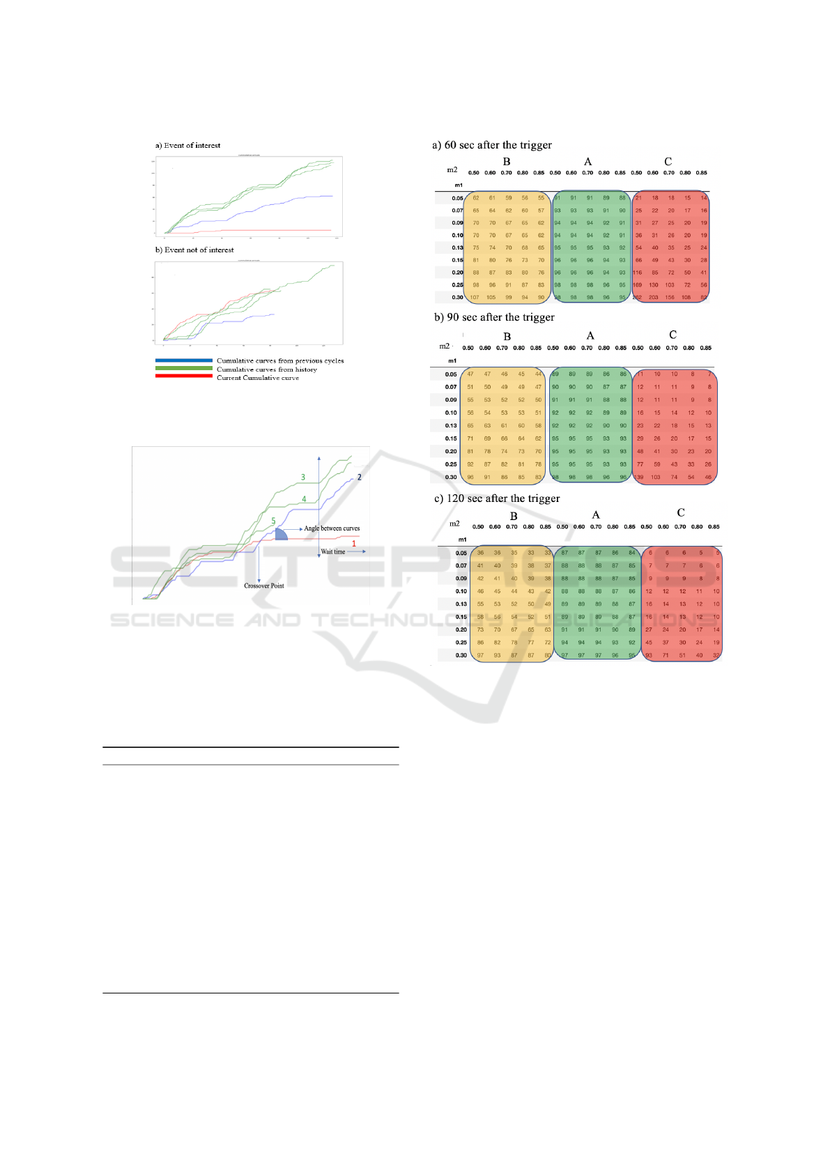
Figure 6: This Figure Shows the Difference between an
Event of Interest and Event Not of Interest. We Plot Cu-
mulative Arrival Volumes Vs Time.
Figure 7: Cumulative Curves of Arrival Volumes Vs Time.
We Use These Curves to Construct Our Feature Set.
time. For each set of detectors, we compute the dis-
tribution of events captured using different thresholds
for feature 1, feature 2 and for different wait times af-
ter the trigger. This is an attempt to determine thresh-
olds for the features in order to capture events of in-
Algorithm 2: Detection Algorithm.
function DETECTION ALGORITHM(volume reduction,
time)
Require: volume reduction - percentage reduction of ar-
rival volume in the cycle. Detector ID - detector at which
interruption happened. ph -phase time - Time at which
reduction happened
for different wait times after the trigger do
Construct cumulative arrival curves based using
current arrivals, history
Construct feature 1, feature 2 from cumulative
arrivals for the wait time as described.
Decision = thresholds(feature1, feature2, wait
time)
end for
Return Decision
end function
Figure 8: Distribution of Events Captured for Different
Thresholds (High Volume Detectors) 60 Sec, 90 Sec, 120
Sec after the Trigger. This Justifies That by Waiting More
Time after the Trigger, We Capture Less Events That Are
Not of Interest.
terest.
Figure 8 shows the distribution of events captured
for different thresholds and wait times 60 sec,90 sec,
120 sec after the trigger for high volume detectors.
We can see that the number of captured events that are
not of interest decrease with an increase in wait time
for the same set of thresholds. This suggests that by
waiting more time after the trigger, we capture fewer
events that are not of interest. Also, the number of
events captured that are not of interest decreases with
an increase in m2 and a decrease in m1 but with the
trade-off is that we miss some of the events of interest.
Figure 9 shows a comparison of the over-
all distribution of events vs events captured when
f eature 1(m1) < 0.09 and feature 2(m2) > 0.7, for
wait times 90 sec after the trigger, for high volume de-
Data Mining Algorithms for Traffic Interruption Detection
111
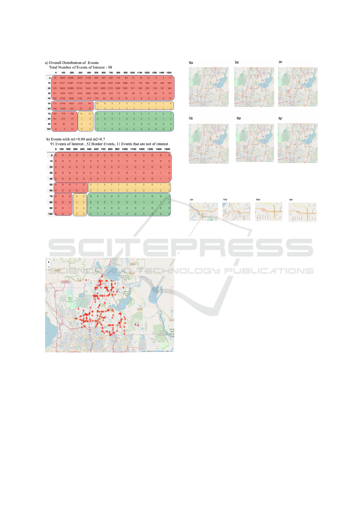
Figure 9: Events Captured for M1 < 0.09 and M2 > 0.7
for Wait Time 90 Sec after the Trigger. 92% of the Events
of Interest, 35% of Border Events, a Minute Percentage of
Events Not of Interest Were Captured. (High Volume De-
tectors).
Figure 10: Locations of All the Events of Interest Gener-
ated from Nov 2018 to Apr 2019. This Plot Shows That
Events Occur More Frequently at Some Intersections When
Compared to Others.
tectors. For this set of thresholds(m1, m2, wait time),
92% of the events of interest, 35% of border events, a
minute percentage of events not of interest were cap-
tured.
Figure 11: Locations of All the Events of Interest Generated
for Each Month Separately from Nov 2018 to Apr 2019.
This Plot Shows the Temporal Consistency of Some Inter-
sections.
Figure 12: Figure Showing an Intersection Where the EOI
Are Occurring Consistently over the Months of January,
February, March and April.
6 SPATIO-TEMPORAL ANALYSIS
OF EVENTS
We also analyze the events of interest with the goal
of discovering human-understandable spatial or tem-
poral patterns. Figure 10 shows plot the of locations
of all the Events of Interest. Each red marker on the
map indicates the location of the intersection where
an event occurred. From the plot we can see that
events are occurring more frequently at some inter-
sections.
6.1 Temporal Patterns
The onus is on temporal pattern discovery to deter-
mine coherent activities at intersections over the pe-
riod of a month. This requires the visualization of
locations of EOI separately for each month. In these
plots, the size of the marker is directly proportional
to the number of events occurring at that particular
intersection. We see from Figure 11 that at some in-
tersections, EOIs occur consistently each month. Fig-
ure 12 shows an example of an intersection where the
EOI occurs consistently over the months of January,
February, March and April. The payoff from tem-
VEHITS 2020 - 6th International Conference on Vehicle Technology and Intelligent Transport Systems
112

poral pattern discovery is the highlighting of problem-
atic intersections in this manner.
Figure 13 shows a set of intersections where inter-
ruptions are occurring consistently every month. At
these intersections, total number of EOI occurred is
greater than 20 and an EOI occurred at least 5 out of
6 months.
6.2 Spatial Patterns
Spatial pattern discovery complements the earlier
case of temporal patterns. Here, we seek to deter-
mine the impact of EOIs at one intersection on a
nearby one. The first step in this process is to de-
rive the network topology. For each intersection, we
derive a set of intersections that are neighbors based
on spatial proximity. The second step is to analyze
the co-occurrences of interruptions in the neighbor-
ing intersections (henceforth termed secondary inter-
ruptions). With this analysis in place, we find that
52 out of 900 events were coincident with—and thus
possibly caused—an interruption in neighboring in-
tersections.
Figure 13: Table Showing a List of Intersections Where To-
tal Number of EOI > 20 and an EOI Occurred at Least 5 out
of 6 Months.
7 CONCLUSIONS
The focus of this work is in the detection and pre-
diction of traffic interruptions without the need for
labeled data (from police reports and the like). Af-
ter first defining events of interest corresponding to
traffic interruptions using large deviations of traf-
fic volumes and the build-up of significant delays,
we constructed an event prediction approach to dis-
cover these interruptions from signalized intersection
datasets. The approach—using time series analysis—
examined (cumulative) approach volumes at intersec-
tions and at specific time points and compared them
to historical (cumulative) approach volumes at similar
time points (hour of the day and/or day of the week).
This proved capable of predicting the occurrence of
events of interest with high accuracy. Finally, we per-
formed a spatio-temporal analysis of the EOIs to find
recurrent patterns in the said events in order to ob-
tain human-understandable summarizations of traffic
interruptions. Our immediate future work will focus
on including police reports and labeled EOIs within
this framework.
ACKNOWLEDGEMENTS
The work was supported in part by NSF CNS
1922782 and by the Florida Department of Trans-
portation (FDOT). The opinions, findings and conclu-
sions expressed in this publication are those of the au-
thors and not necessarily those of FDOT.
REFERENCES
Ahmed, F. and Hawas, Y. E. (2012). A threshold-based real-
time incident detection system for urban traffic net-
works. Procedia - Social and Behavioral Sciences,
48:1713 – 1722. Transport Research Arena 2012.
Balke, K., Dudek, C. L., and Mountain, C. E. (1996). Using
probe-measured travel time to detect major freeway
incidents in houston, texas. Transportation Research
Record, No, 1554:213–220.
Gu, Y., Qian, Z. S., and Chen, F. (2016). From twitter to de-
tector: Real-time traffic incident detection using social
media data. Transportation research part C: emerging
technologies, 67:321–342.
Jeong, Y.-S., Castro-Neto, M., Jeong, M. K., and Han, L. D.
(2011). A wavelet- based freeway incident detection
algorithm with adapting threshold parameters. Trans-
portation Research Part C: Emerging Technologies,
19(1):1–19.
Jin, X., Cheu, R. L., and Srinivasan, D. (2002). Devel-
opment and adaptation of constructive probabilistic
neural network in freeway incident detection. Trans-
portation Research Part C: Emerging Technologies,
10(2):121–147.
Lee, J.-T. and Taylor, W. C. (1999). Application of a dy-
namic model for arterial street incident detection. ITS
Journal - Intelligent Transportation Systems Journal,
5(1):53–70.
Lin, W.-H. and Daganzo, C. F. (1997). A simple de-
tection scheme for delay-inducing freeway incidents.
Transportation Research Part A: Policy and Practice,
31(2):141 – 155.
Lingras, P. and Adamo, M. (1996). Average and peak traf-
ficvolumes: Neural nets, regression, and factor ap-
proaches, jour-nal of computing in civil engineering.
ASCE, 10(4):300–6.
Mouskos, K. C., Niver, E., Lee, S., Batz, T., and Dwyer,
P. (1999). Transportation operation coordinating com-
mittee system for managing incidents and traffic: eval-
uation of the incident detection system. Transporta-
tion Research Record, No, 1679:50–57.
Park, H. and Haghani, A. (2016). Real-time prediction of
secondary incident occurrences using vehicle probe
data. Transportation Research Part C: Emerging
Technologies, 70:69–85.
Data Mining Algorithms for Traffic Interruption Detection
113

Parkany, E. and Xie, C. (2005). A complete review of in-
cident detection algorithms & their deployment: what
works and what doesn’t. TRR.
Teng, H. and Qi., Y. (2003). Application of wavelet tech-
nique to freeway incident detection. Transporta-
tion Research Part C: Emerging Technologies, 11(3-
4):289–308.
Williams, B. M. and Guin, A. (2007). Traffic management
center use of incident detection algorithms: Findings
of a nationwide survey. Trans. Intell. Transport. Sys.,
8(2):351–358.
Yang, H., Wang, Z., Xie, K., and Dai, D. (2017). Use
of ubiquitous probe vehicle data for identifying sec-
ondary crashes. Transportation research part C:
emerging technologies, 82:138–160.
VEHITS 2020 - 6th International Conference on Vehicle Technology and Intelligent Transport Systems
114
