Decision Guidance on Software Feature Selection to Maximize the

Benefit to Organizational Processes

Fernando Boccanera and Alexander Brodsky

Computer Science Department, George Mason University, Virginia, U.S.A.

Keywords: Decision Guidance System, Decision Support System, Software Release Schedule, Optimization,

Mixed-Integer Linear Programming.

Abstract: Many software development projects fail because they do not deliver sufficient business benefit to justify the

investment. Existing approaches to estimating business benefit of software adopt unrealistic assumptions

which produce imprecise results. This paper focuses on removing this limitation for software projects that

automate business workflow processes. For this class of projects, the paper proposes a new approach and a

decision-guidance framework to select and schedule software features over a sequence of software releases

as to maximize the net present value of the combined cash flow of software development as well as the

improved organizational business workflow. The uniqueness of the proposed approach is in precise modelling

of the business workflow and the savings achieved by deploying new software functionality.

1 INTRODUCTION

Many software development projects fail because

they do not deliver much business benefit. Research

has shown that 25% of projects fail and another 25%

do not provide any return on investment (Pucciarelli

& Wiklund, 2009). Of those projects that do not fail,

45% of the functionality is never used, resulting in

zero business value (The Standish Group, 2014). This

has led to an increasing understanding that “value

creation is the final arbiter of success for investments

of scarce resources; and far greater sophistication

than in the past is now evident in the search for value”

(Boehm & Sullivan, 2000).

This paper focuses on maximizing the business

value for a class of software projects that automate

Business Workflow Processes (BWP). It proposes a

new approach and a decision-guidance framework to

select and schedule software features over a sequence

of software releases as to maximize the return on

investment (ROI). The uniqueness of the proposed

approach is that ROI analysis is based on precise

modelling of the BWP and the savings achieved by

deploying new software functionality.

There has been extensive work on the selection

and scheduling of software functionality to increase

the business value of software investments, among

them, the highly influential Incremental Funding

Methodology (IFM) approach (M. Denne & Cleland-

Huang, 2004), (Cleland-Huang & Denne, 2005),

(Mark Denne & Cleland-Huang, 2003). IFM’s

approach is to deliver software functionality, called

features, as early as possible in order to maximize

their business value. It assumes a software

development life cycle that delivers software

continuously and iteratively in releases, in line with

modern Agile methodologies like Scrum.

Another approach called F-EVOLVE* (Maurice

et al., 2006), is an iterative and evolutionary approach

that facilitates the involvement of stakeholders to

achieve increments (releases) that result in the highest

degree of satisfaction among different stakeholders.

The approach provides a decision support for the

generation and selection of release plan alternatives.

A third approach (Van den Akker et al., 2005),

applies integer linear programming to maximize the

revenue.

However, estimating the business benefit of a

software release is challenging. All existing

approaches use cash flow as a metric for business

benefits, but their estimations are inaccurate. IFM and

Van den Akker et al. assume that cash flow

estimations are provided externally, that is, they are

not part of the approach, while F-EVOLVE* gets

estimates from multiple stakeholders and weights

them according to the perceived importance of each

stakeholder. Also, they require the estimation of cash

Boccanera, F. and Brodsky, A.

Decision Guidance on Software Feature Selection to Maximize the Beneﬁt to Organizational Processes.

DOI: 10.5220/0009400403810395

In Proceedings of the 22nd International Conference on Enterprise Information Systems (ICEIS 2020) - Volume 1, pages 381-395

ISBN: 978-989-758-423-7

381

flows at the software feature level which is

challenging due to the difficulty of drawing a direct

correlation between a particular business benefit, like

a reduction in cost, and a specific piece of software.

Some researchers have acknowledged this difficulty,

e.g., (Devaraj & Kohli, 2002) noted that “the

principal issue encountered is whether we can isolate

the effect of IT on firm performance. It does not have

an easy answer, because it means disentangling the

effect of IT from various other factors such as

competition, economic cycle, capacity utilization,

and many other context-specific issues.”

Existing value-based approaches other than the

three mentioned were not considered because they are

not comprehensive. For example, (Riegel & Doerr,

2014) developed heuristics that can be used to

optimize requirements selection, but their cost metric

only involves elicitation, not development. (Hannay

et al., 2017) used benefit points as a metric for

business value but did not propose a release

scheduling approach. (Elsaid et al., 2019) used rule-

based fuzzy logic to prioritize requirements but did

not consider the development cost.

A significant pitfall of existing value-based

release scheduling approaches like IFM, F-

EVOLVE* and Van den Akker et al. is that each and

every dollar of cash flow needs to be allocated to one

and only one feature. This is not a realistic

assumption because often, realizing a business

benefit does require the implementation of more than

one software feature. Another pitfall is that the cash

flow of the business benefit (revenue or savings) and

the cost of development are combined into a single

value. This conceals the cost of development from the

decision maker and force development cost changes

to be applied first to the external cash flows prior to

being used in the model.

Because of these pitfalls, the estimation of

business benefits is often based on a guesswork and,

as a result, is inaccurate. This inaccuracy, together

with the estimation of business benefits being

external to the methodology, are the limitations of

existing value-based approaches.

The focus of this paper is addressing the

limitations of the existing value-based release

scheduling approaches for the class of software

projects that improve a Business Workflow Process

(BWP). We address the limitations by proposing a

decision-guidance framework that is more precise

than existing approaches because it is based on a

formal model of the BWP and its evolution following

the implementation of software features.

The key idea, which is also unique, is that the

implementation of software features allows

improvements in the BWP, which lead to a reduction

in cost. As a consequence of this idea, the business

benefit is not attributed to individual features in silos

like in the current approaches, but rather to the

synergetic effect of multiple interrelated features on

the reduction of the overall cost of the BWP. The

proposed approach moves the benefit estimation from

a guesswork to a systematic model-based

methodology, which, we believe, will result in

considerably higher return on software investment.

More specifically, the contributions of this paper

are threefold. We (1) develop a formal optimization

model and solution based on a reusable library of

analytical component models; (2) develop a decision

guidance system and methodology for software

release scheduling; and (3) demonstrate the

methodology using an example from the U.S. Patent

and Trademark Office.

The first contribution, the formal model, captures

the entire space of alternatives for BWP networks

which produce some output items from input items

(e.g., documents, requests, approvals, etc.). Every

process in a BWP hierarchy is described, recursively,

as a flow of items through a number of sub-processes.

Some parent processes require an exclusive OR

choice among their children sub-processes

(introducing alternatives), while others require all

their children sub-processes to be activated.

The formal optimization model decides on (1)

which interdependent software features are to be

implemented and in which software release, and (2)

which specific alternatives of the BWP network are

to be activated for each software release over the

investment horizon. To be activated, atomic

processes in the BWP hierarchy may require new

inter-dependent software features to be implemented.

Improvements in the BWP are measured as cash

flows and their associated Net Present Value (NPV).

Cash flows are calculated to represent the ongoing

costs of the BWP, as well as software development.

Each potential software release schedule impacts the

cash flow and results in a different NPV. The formal

optimization problem is to minimize the NPV of the

combined cash flow of the BWP plus the software

cost, while satisfying the constraints of (1) feature-to-

release allocation, (2) dependencies among features,

and (3) business processes activation.

As a second contribution, we develop a Decision

Guidance System (DGS) and methodology that are

centered around solving the optimization model and

producing an optimal release sequence. The DGS is

based on the formal model and is implemented in the

Decision Guidance Analytics Language (DGAL)

(Alexander Brodsky & Luo, 2015) within Unity

ICEIS 2020 - 22nd International Conference on Enterprise Information Systems

382

(Nachawati et al., 2016), a generic platform for the

creation and execution of decision guidance systems.

Finally, to demonstrate the approach, we show a

simplified example from the United States Patent and

Trademark Office, with all the essential components.

This paper is organized as follows: Section 2

intuitively explains the proposed approach through an

example; Section 3 describes the formal model;

Section 4 discusses the methodology and decision

guidance system; Section 5 is an example of the

approach; and, Section 6 provides concluding

remarks and briefly describes future research.

2 INTUITIVE EXPLANATION OF

THE RELEASE SCHEDULING

APPROACH

We first describe the proposed approach intuitively

through an example. The goal is to maximize the

business value of an investment in an information

system that improves a business process.

BWP Modelling

Consider an organization, like the United States

Patent Office, which processes applications for

patents. Consider a simplified and partial version of

the business process workflow, depicted in Figure 1.

The process starts with Application Intake (A), which

takes a User Application and either accepts it by

producing a Compliant Application or rejects it by

producing a Non-compliance Notice. Compliant

applications go through Adjudication (B) and then

Adjudication Review (C), which produces an

Adjudicated Application Letter.

A.Application

Intake

B.

Adjudication

C.

Adjudication

Review

Compliant

Application

Adjudicated

Application

Adjudicated

Application

Letter

User

Application

Non

Compliance

Notice

root:ServiceNetwork(type:AND)

Figure 1: Simplified Patent Adjudication BWP.

Let us assume that initially, processes A, B and C

are manual, and the Patent Office is considering

implementing a software system to automate these

processes to save cost. To reason about possible

alternatives for automation, the Office creates the

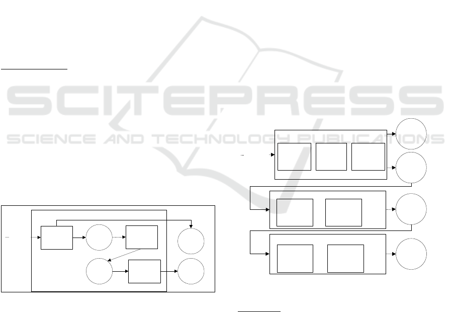
diagram shown in Figure 2. In it, process A has three

alternatives; AA (Manual Application Intake), AB

(Electronic Application Intake) and AC (Self-service

Application Intake), where AA is the initial manual

process and AB and AC are increasingly automated

alternatives of A. Similarly, for B, BA is the initial

manual process while BB is its automated alternative

and for C, CA is manual while CB is its automated

alternative. In essence, Figures 1 and 2 show all

possible configurations of the BWP, composed of a

combination of alternatives to processes A, B and C.

Initially there is no software system, consequently

the BWP configuration is made of manual processes

AA (Manual Application Intake), BA (Manual

Adjudication) and CA (Manual Adjudication

Review). As the software system is implemented, the

BWP configuration changes to take advantage of

more efficient processes; AA transitions to AB

(Electronic Application Intake), BA transitions to BB

(Electronic Adjudication), etc…

We model the BWP as a Service Network (SN)

(A. Brodsky et al., 2017), which is a “network of

service-oriented components that are linked together

to produce products”. Figure 1 depicts the root

Service Network, while Figure 2 details its

subservices A, B and C. Because the root service

requires subservices A, B and C, we call this an AND-

type service. Whereas, because service A requires

only one of subservices AA, AB or AC, service A is

an OR-type. Services B and C are also OR-types

while all the other subservices are atomic.

Non‐

compliance

Notice

Compliant

Application

AA.

Manual

Application

Intake

AB.

Electronic

Application

Intake

AC.

Self‐service

Application

Intake

User

Ap pl icati on

Adjudicated

Application

B.AdjudicationReview(type:OR)

BA.

Manua l

Adjudication

BB.

Electronic

Adjudication

Adjudicated

Application

Letter

C.AdjudicationReview(type:OR)

Manua l

Adjudication

Review

CB.

Electronic

Adjudication

Review

A.ApplicationIntake(type:OR)

(A)

(B)

(C)

Figure 2: BWP Composite Processes A, B and C.

BWP Cost

Different automation alternatives potentially reduce

the cost of the BWP for patent adjudication. Cost

savings may be due to reduction of the amount of

manual labor or utilization of less costly labor.

However, automated process alternatives require the

implementation of specific software functionality

called features. For example, process alternative AB

(Electronic Application Intake) requires business

feature BF1 which is the capability to create and edit

Decision Guidance on Software Feature Selection to Maximize the Beneﬁt to Organizational Processes

383

an electronic application. Table 1 shows which

features are required for each process alternative,

where BF is a business feature and TF is a technical

feature.

Our approach uses the cost reduction of

automated processes to precisely calculate the

business value of software. In our approach, there is

no need to estimate the cash flow at the feature level;

a feature is just an enabler of a change in the BWP

configuration.

Table 1: Process alternatives and required software

features.

Process

Alternative

Required

Feature

Functionality

one

AB BF1 Capability to create and

edit an electronic appl.

AC BF4 Capability to allow an

Applicant to submit an

application on-line

one

BB BF2 Capability to annotate

aspects of the applicatio

that pass or don't pass

udication rules

one

CB BF3 Capability to review

adjudication decision

and annotate issues that

don't pass review

Software Features

Features must be scheduled over a sequence of

releases. The set of features implemented in a

particular release incur a development cost and

enables a set of candidate BWP configurations, which

in turn, are associated with labor cost savings. A

software release schedule is a table of all releases and

the features planned to be implemented in each

release. The choice of features to be implemented in

a particular release is constrained by the fact that

features require varying levels of effort, but the

development team has a fixed capacity. This means

that the total effort scheduled for any release cannot

exceed the capacity of the development team.

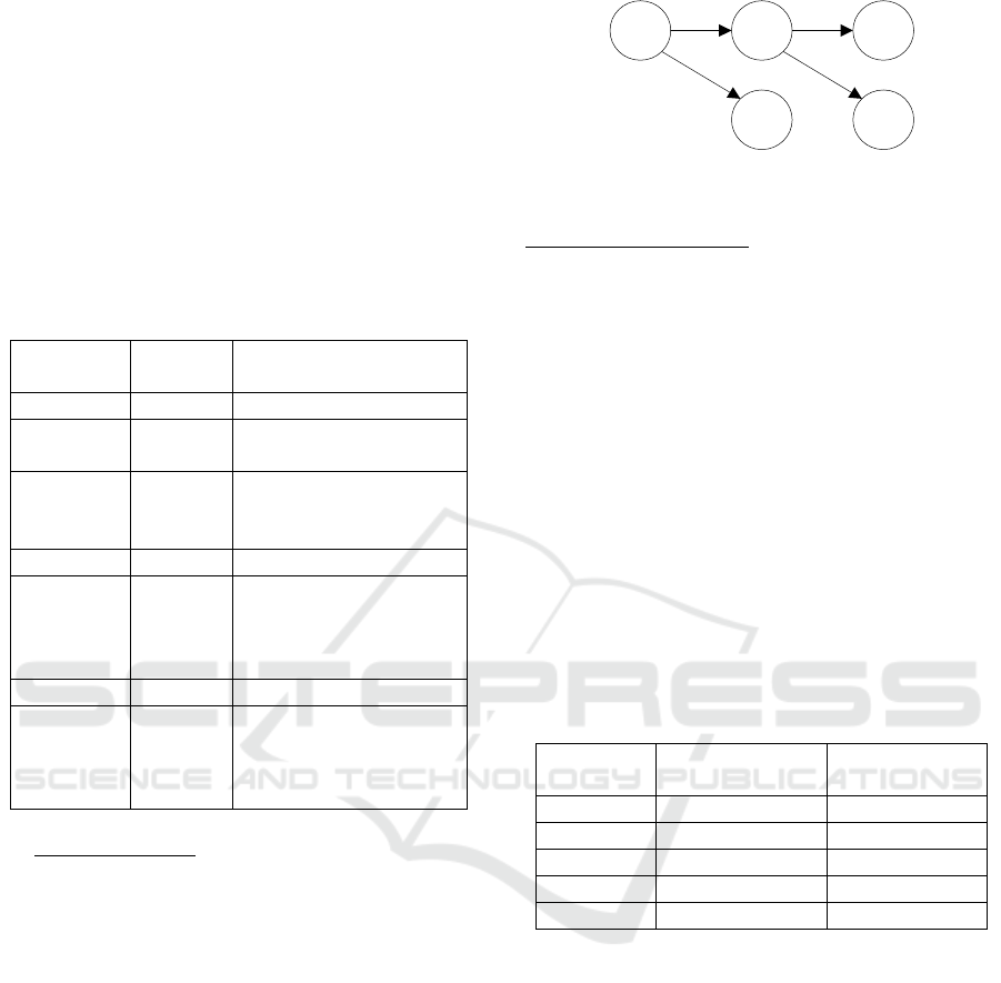
Another constraint is that features have

interdependencies that form a graph. Figure 3 depicts

the dependency graph for our example. It shows that

business feature BF1 is a prerequisite for BF2 and

BF4 while technical feature TF1 is a prerequisite for

BF1 and BF3.

TF1 BF1 BF2

BF3 BF4

Figure 3: Dependency Graph.

Best BWP Configuration

There are many possible mappings between features,

releases and BWP configurations. One such mapping

is the release sequence shown in Table 2. During

release 1, TF1 and BF1 are being implemented but

still not available. Consequently, the best BWP

configuration is AA, BA, and CA because, according

to Table 1, it does not require any software feature.

During release 2, BF3 is being implemented but still

not available, therefore, the set of completed features

is {TF1, BF1} consequently, the best BWP

configuration is AB, BA and CA because feature

BF1, according to Table 1, enables process AA to

transition to AB. The same rationale applies to

releases 3 and 4. After release 4 all features are

implemented and the best configuration, which is also

the least costly, is AC, BB and CB.

Table 2: Example of software release schedule and best

BWP configuration.

Software

Release #

Features being

implemented

Best BWP

Configuration

1 TF1, BF1 AA, BA, CA

2 BF3 AB, BA, CA

3 BF2 AB, BA, CB

4 BF4 AB, BB, CB

After 4 AC, BB, CB

Note that the feature sequence in Table 2 complies

with the dependency graph in Figure 3 because TF1

and BF1 are implemented before BF2, BF3 and BF4.

Also, TF1 is implemented in the same release as BF1.

Every software release schedule and related BWP

configuration, such as the one depicted in Table 2,

corresponds to a cash flow and the NPV associated

with (1) the cost of software development, and (2) the

cost of running the BWP. Our problem is finding a

software release schedule and BWP configuration

that maximizes the overall NPV, subject to

constraints such as the BWP space of alternatives, the

required software features, the interdependencies

among features, the one-to-one mapping between

features and releases and the capacity of the

development team.

ICEIS 2020 - 22nd International Conference on Enterprise Information Systems

384

3 FORMAL MODEL

3.1 Model Introduction

The release scheduling problem formulation in linear

programming is:

𝑀𝑎𝑥



𝑂



𝑃,𝐷𝑉



𝑠.𝑡. 𝐶𝑃,𝐷𝑉

Where:

P is a set of parameters,

DV is a set of decision variables,

𝐶



𝑃,𝐷𝑉



is a predicate, expressed as a function of

parameters 𝑃 and decision variables 𝐷𝑉, that

need to be satisfied, and

𝑂



𝑃,𝐷𝑉



is the NPV metric, expressed as a

function of P and DV

The components of the optimization problem are

described using the ReleaseScheduling

formalization, which is a tuple ⟨Parameters,

DecisionVariables, Computation, Constraints,

InterfaceMetrics⟩, detailed in section 3.2. At a high

level, the ReleaseScheduling formalization is

described in Figure 4 as a hierarchy of components.

Release

Scheduling

Business

Service

Network

Software

Development

ServicesSet Service

ANDService

InputDrivenAtomic

ORService

Figure 4: Hierarchy of the Formalizations of the Release

Scheduling Model.

The hierarchy in Figure 4 establishes a parent-

child relationship where the child inherits all

formalizations from the parent and the parent has

access to all the formalizations of the child. For

example, ReleaseScheduling is the parent of Business

Service Network (BSN), consequently the BSN tuple

is available to ReleaseScheduling and BSN inherits

Parameters, DecisionVariables, Computations and

InterfaceMetrics from ReleaseScheduling.

In the next sections we describe the components

of the Release Scheduling formalization hierarchy in

details.

3.2 Release Scheduling Formalization

ReleaseScheduling (RSch) formalization is a tuple

⟨Parameters, DecisionVariables, Computation,

Constraints, InterfaceMetrics⟩

where:

Parameters, also denoted Parm, is a tuple ⟨Features,

TH, DiscountRate, ReleaseInfo, BSN.Parameters,

SWD.Parameters⟩

Features is a tuple ⟨BF, TF, DG, FS ⟩ where:

 BF is a set of business features

 TF is a set of technical features, such that

𝐵𝐹∩𝑇𝐹 ∅

 DG, (Dependency Graph), is a partial order over

F = BF ∪ TF, (f

, f

) ∈ DG also denoted f

≺ f

means that f

is dependent on f

, that is, feature f

a pre-requisite for feature f

 𝑭𝑺:𝐹 → ℝ



is a function described as follows:



∀ 𝑓∈𝐹



,𝐹𝑆𝑓 gives the size, in effort point, of

each feature 𝑓.

 TH is the time horizon for analysis in days

 DiscountRate is the daily rate to discount cash

flows.

 ReleaseInfo is a tuple ⟨NR, RD ⟩, where:

 NR is the number or releases

 𝑹𝑫∶



1..𝑁𝑅



→ ℝ



is a function described as

follows:



∀ 𝑟∈



1..𝑁𝑅





,𝑅𝐷



𝑟



gives the

maximum duration in days for release 𝑟.

 BSN.Parameters is defined in section 3.3

 SWD.Parameters is defined in section 3.8

DecisionVariables, also denoted DV, is a tuple

⟨

𝐼𝐵𝐹,𝐼𝑇𝐹,𝐵𝑆𝑁.𝐷𝑒𝑐𝑖𝑠𝑖𝑜𝑛𝑉𝑎𝑟𝑖𝑎𝑏𝑙𝑒𝑠,

𝑆𝑊𝐷.𝐷𝑒𝑐𝑖𝑠𝑖𝑜𝑛𝑉𝑎𝑟𝑖𝑎𝑏𝑙𝑒𝑠

⟩

where:

 𝑰𝑩𝑭∶



1..𝑁𝑅



→2



is a function described as

follows:



∀ 𝑟∈



1..𝑁𝑅





,𝐼𝐵𝐹𝑟 gives a set of

business features planned to be implemented in

release 𝑟.

 𝑰𝑻𝑭∶



1..𝑁𝑅



→2



is a function described as

follows:



∀ 𝑟∈



1..𝑁𝑅





,𝐼𝑇𝐹𝑟 gives a set of

technical features planned to be implemented in

release 𝑟.

 𝑩𝑺𝑵.𝑫𝒆𝒄𝒊𝒔𝒊𝒐𝒏𝑽𝒂𝒓𝒊𝒂𝒃𝒍𝒆𝒔 is defined in section

3.3.

 𝑺𝑾𝑫.𝑫𝒆𝒄𝒊𝒔𝒊𝒐𝒏𝑽𝒂𝒓𝒊𝒂𝒃𝒍𝒆𝒔 is defined in section

3.8.

Computation

1. Let 𝑆𝑜𝐹𝑎𝑟𝐼𝐵𝐹:



1..𝑁𝑅1



→2



be a function

described as follows:



∀ 𝑟∈



1..𝑁𝑅 1





𝑆𝑜𝐹𝑎𝑟𝐼𝐵𝐹𝑟 gives the set of all business features

Decision Guidance on Software Feature Selection to Maximize the Beneﬁt to Organizational Processes

385

implemented up to release 𝑟 or the period after the

last release, computed as follows:

𝑆𝑜𝐹𝑎𝑟𝐼𝐵𝐹



𝑟







𝐼𝐵𝐹



𝑖







2. Let 𝐶𝑜𝑚𝑏𝑖𝑛𝑒𝑑𝐶𝑎𝑠ℎ𝐹𝑙𝑜𝑤:



1..𝑇𝐻



→ℝ be a

function described as follows:



∀ 𝑑∈



1..𝑇𝐻





,𝐶𝑜𝑚𝑏𝑖𝑛𝑒𝑑𝐶𝑎𝑠ℎ𝐹𝑙𝑜𝑤𝑑 gives the

combined income/expenditure of both the Business

Service Network and the Software Development,



∀ 𝑑∈



1..𝑇𝐻





, computed as follows:

𝐶𝑜𝑚𝑏𝑖𝑛𝑒𝑑𝐶𝑎𝑠ℎ𝐹𝑙𝑜𝑤



𝑑



𝐵𝑆𝑁.𝐼𝑀.𝐶𝑎𝑠ℎ𝑓𝑙𝑜𝑤



𝑑



 𝑆𝑊𝐷.𝐼𝑀.𝐶𝑎𝑠ℎ𝐹𝑙𝑜𝑤



𝑑



where:

 BSN.IM.CashFlow is defined in section

BSN.InterfaceMetrics of section 3.3

 SWD.IM.CashFlow is defined in section

Software.InterfaceMetrics of section 3.8.

Note that a negative cash flow means that it is a cash

outflow.

3. Let 𝑇𝑖𝑚𝑒𝑊𝑖𝑛𝑑𝑜𝑤𝑁𝑃𝑉:



1..𝑇𝐻



→ℝ be a

function described as follows:



∀ 𝑑∈



1..𝑇𝐻





𝑇𝑖𝑚𝑒𝑊𝑖𝑛𝑑𝑜𝑤𝑁𝑃𝑉𝑑 gives the Net Present

Value (NPV) of the CombinedCashFlow for the

time investment window1..𝑑, computed as

follows:

𝑇𝑖𝑚𝑒𝑊𝑖𝑛𝑑𝑜𝑤𝑁𝑃𝑉



𝑑





𝐶𝑜𝑚𝑏𝑖𝑛𝑒𝑑𝐶𝑎𝑠ℎ𝐹𝑙𝑜𝑤𝑖



1𝐷𝑖𝑠𝑐𝑜𝑢𝑛𝑡𝑅𝑎𝑡𝑒









4. Let F = BF ∪ TF

5. Let 𝐼𝐹



𝑟



 𝐼𝐵𝐹



𝑟



∪𝐼𝑇𝐹



𝑟



,∀𝑟∈



1..𝑁𝑅





6. FeatureSetsForReleasesArePairwiseDisjoint

constraint is:



∀ 𝑖,𝑗,∈



1..𝑁𝑅



,𝑖𝑗



,𝐼𝐹



𝑖



∩𝐼𝐹



𝑗



∅

7. DependencyGraphIsSatisfied constraint is:

(∀𝑟∈



1..𝑁𝑅







∀ 𝑓



,𝑓



∈ 𝐹



𝑓



≺𝑓



∧𝑓



∈𝐼𝐹



𝑟



→𝑓



∈



𝐼𝐹



𝑖









Constraints

FeatureSetsForReleasesArePairwiseDisjoint is

defined in computation #6 above.

DependencyGraphIsSatisfied is defined in

computation #7 above.

BSN.Constraints is defined in section 3.3.

SWD.Constraints is defined in section 3.8.

InterfaceMetrics, also denoted IM, is a tuple

⟨

𝑆𝑜𝐹𝑎𝑟𝐼𝐵𝐹,𝐶𝑜𝑚𝑏𝑖𝑛𝑒𝑑𝐶𝑎𝑠ℎ𝐹𝑙𝑜𝑤,

𝑇𝑖𝑚𝑒𝑊𝑖𝑛𝑑𝑜𝑤𝑁𝑃𝑉,𝐵𝑆𝑁.𝐼𝑛𝑡𝑒𝑟𝑓𝑎𝑐𝑒𝑀𝑒𝑡𝑟𝑖𝑐𝑠,

𝑆𝑊𝐷.𝐼𝑛𝑡𝑒𝑟𝑓𝑎𝑐𝑒𝑀𝑒𝑡𝑟𝑖𝑐𝑠

⟩

where:

 𝑪𝒐𝒎𝒃𝒊𝒏𝒆𝒅𝑪𝒂𝒔𝒉𝑭𝒍𝒐𝒘 is defined in computation

#2 above.

 𝑻𝒊𝒎𝒆𝑾𝒊𝒏𝒅𝒐𝒘𝑵𝑷𝑽 is defined in computation #3

above.

 BSN.InterfaceMetrics is defined in section 3.3

 SWD.InterfaceMetrics is defined in section 3.8

3.3 Business Service Network

Formalization

A Business Service Network (BSN) is the formal

equivalent of the BWP.

BusinessServiceNetwork formalization, also

denoted BSN, is a tuple ⟨Parameters,

DecisionVariables, Computation, Constraints,

InterfaceMetrics⟩, where:

Parameters, also denoted Parm, is a tuple

⟨LaborRates, LaborPaySched, BSNDemand,

ServicesSet, rootID⟩,

where:

 LaborRates is a tuple ⟨LR, Rate⟩ where:

 LR is a set of labor roles

 𝑹𝒂𝒕𝒆:𝐿𝑅→ℝ



is a function described as follows:

(∀ 𝑙 ∈ 𝐿𝑅,𝑅𝑎𝑡𝑒𝑙 gives the daily rate for labor

role 𝑙.

 LaborPaySched, the labor cost payment schedule,

is a tuple

⟨

𝑁𝐿𝑃,𝐿𝑎𝑏𝑜𝑟𝑃𝑎𝑦𝐷𝑎𝑦𝑠

⟩

where:

 𝑵𝑳𝑷∈ℝ



is the number of labor payments over

the entire time horizon

 𝑳𝒂𝒃𝒐𝒓𝑷𝒂𝒚𝑫𝒂𝒚:



1..𝑁𝐿𝑃



→ 1..𝑇𝐻 is a

function described as follows: (∀ 𝑝∈



1..𝑁𝐿𝑃



,𝐿𝑎𝑏𝑜𝑟𝑃𝑎𝑦𝐷𝑎𝑦𝑝 gives the day,

relative to the first day of the time horizon, on

which a payment 𝑝 is made.

 BSNDemand, is a tuple

⟨

𝐵𝑆𝑁𝐼,𝐵𝑆𝑁𝑂,𝐷𝑒𝑚𝑎𝑛𝑑

⟩

where:

 BSNI is a set of input items ids that have to be

processed by the Service Network.

 BSNO is a set of output items ids that have to be

produced by the Service Network.

 𝑫𝒆𝒎𝒂𝒏𝒅:𝐵𝑆𝑁𝐼

⋃

𝐵𝑆𝑁𝑂→ℝ



is a function

described as follows: ∀ 𝑗∈𝐵𝑆𝑁𝐼

⋃

𝐵𝑆𝑁𝑂,

𝐷𝑒𝑚𝑎𝑛𝑑𝑗 gives for every item 𝑗, the required

processing throughput per hour.

 ServicesSet is the set of all services in the Service

Network, defined in section 3.4.

 𝒓𝒐𝒐𝒕𝑰𝑫 is the id of the Service, in the ServicesSet,

which is designated to be the “root”. The definition

of a Service is given in section 3.4.

ICEIS 2020 - 22nd International Conference on Enterprise Information Systems

386

DecisionVariables is the set



𝑠.𝐷𝑒𝑐𝑖𝑠𝑖𝑜𝑛𝑉𝑎𝑟𝑖𝑎𝑏𝑙𝑒𝑠

𝑠∈𝑆𝑒𝑟𝑣𝑖𝑐𝑒𝑠𝑆𝑒𝑡. See

section 3.4.

Computation

Let root be a Service in ServicesSet with id=rootid

𝐵𝑆𝑁𝐷𝑒𝑚𝑎𝑛𝑑𝐼𝑠𝑆𝑎𝑡𝑖𝑠𝑓𝑖𝑒𝑑 constraint:



∀ 𝑖∈𝐵𝑆𝑁𝐼



∀ 𝑟∈



1..𝑁𝑅1



𝑆𝑒𝑟𝑣𝑖𝑐𝑒.𝐼𝑀.𝐼𝑛𝑝𝑢𝑡𝑇ℎ𝑟𝑢



𝑟𝑜𝑜𝑡𝐼𝐷,𝑖,𝑟



𝐷𝑒𝑚𝑎𝑛𝑑



𝑖



 𝑆𝑒𝑟𝑣𝑖𝑐𝑒.𝐼𝑀.𝐼𝑛𝑝𝑢𝑡𝑇ℎ𝑟𝑢



𝑟𝑜𝑜𝑡𝐼𝐷,𝑟



is defined

in section 3.5

𝐵𝑆𝑁𝑆𝑢𝑝𝑝𝑙𝑦𝐼𝑠𝑆𝑎𝑡𝑖𝑠𝑓𝑖𝑒𝑑 constraint:



∀ 𝑜∈𝐵𝑆𝑁𝑂



∀ 𝑟∈



1..𝑁𝑅 1



𝑆𝑒𝑟𝑣𝑖𝑐𝑒.𝐼𝑀.𝑂𝑢𝑡𝑝𝑢𝑡𝑇ℎ𝑟𝑢



𝑟𝑜𝑜𝑡𝐼𝐷,𝑜,𝑟



𝐷𝑒𝑚𝑎𝑛𝑑



𝑜



 𝑆𝑒𝑟𝑣𝑖𝑐𝑒.𝐼𝑀.𝑂𝑢𝑡𝑝𝑢𝑡𝑇ℎ𝑟𝑢



𝑟𝑜𝑜𝑡𝐼𝐷,𝑟



defined in section 3.5

Let 𝐵𝑆𝑁𝐶𝑜𝑠𝑡𝐹𝑜𝑟𝐷𝑎𝑦∶



1..𝑇𝐻



→ℝ



be a

function described as follows: ∀ 𝑑∈



1..𝑇𝐻



,

𝐵𝑆𝑁𝐶𝑜𝑠𝑡𝐹𝑜𝑟𝐷𝑎𝑦



𝑑



gives the service network

labor cost accrued for day 𝑑 computed as:

𝐵𝑆𝑁𝐶𝑜𝑠𝑡𝐹𝑜𝑟𝐷𝑎𝑦



𝑑



𝑆𝑒𝑟𝑣𝑖𝑐𝑒.𝐼𝑀.𝐶𝑜𝑠𝑡𝑃𝑒𝑟𝐷𝑎𝑦



𝑟𝑜𝑜𝑡𝐼𝐷,𝑟



Where:

 r is the release period (or period after the last

release) where day d appears, i.e.,

𝑆𝑊𝐷.𝐼𝑀.𝑓𝑖𝑟𝑠𝑡𝐷𝑎𝑦



𝑟



𝑑𝑆𝑊𝐷.𝐼𝑀.𝑙𝑎𝑠𝑡𝐷𝑎𝑦



𝑟



 𝑆𝑒𝑟𝑣𝑖𝑐𝑒.𝐼𝑀.𝐶𝑜𝑠𝑡𝑃𝑒𝑟𝐷𝑎𝑦



𝑟𝑜𝑜𝑡𝐼𝐷,𝑟



defined in section 3.5

 𝑆𝑊𝐷.𝐼𝑀.𝑓𝑖𝑟𝑠𝑡𝐷𝑎𝑦 and 𝑆𝑊𝐷.𝐼𝑀.𝑙𝑎𝑠𝑡𝐷𝑎𝑦 are

defined in section 3.8.

Let 𝐵𝑆𝑁𝑃𝑎𝑦𝑚𝑒𝑛𝑡:



1..𝑁𝐿𝑃



→ℝ be a function

described as follows:



∀ 𝑝∈



1..𝑁𝐿𝑃





𝐵𝑆𝑁𝑃𝑎𝑦𝑚𝑒𝑛𝑡



𝑝



gives the service network labor

payment in dollars, for each scheduled payment 𝑝,

computed as:

𝐵𝑆𝑁𝑃𝑎𝑦𝑚𝑒𝑛𝑡𝑝



⎩

⎪

⎨

⎪

⎧

𝐵𝑆𝑁𝐶𝑜𝑠𝑡𝐹𝑜𝑟𝐷𝑎𝑦



𝑑













∀𝑝1



𝐵𝑆𝑁𝐶𝑜𝑠𝑡𝐹𝑜𝑟𝐷𝑎𝑦



𝑑



∀𝑝



2..𝑁𝐿𝑃







Let 𝐶𝑎𝑠ℎ𝐹𝑙𝑜𝑤∶



1..𝑇𝐻



→ℝ



be a function

described as follows:



∀ 𝑑∈



1..𝑇𝐻





,𝐶𝑎𝑠ℎ𝐹𝑙𝑜𝑤



𝑑



gives the cash flow for

the entire Business Service Network for day 𝑑,

computed as follows:

𝑖𝑓 𝑑𝐿𝑎𝑏𝑜𝑟𝑃𝑎𝑦𝐷𝑎𝑦



𝑝



𝑓𝑜𝑟 𝑠𝑜𝑚𝑒 𝑝𝑎𝑦𝑚𝑒𝑛𝑡 𝑝

Then 𝐶𝑎𝑠ℎ𝐹𝑙𝑜𝑤



𝑑



 𝐵𝑆𝑁𝑃𝑎𝑦𝑚𝑒𝑛𝑡



𝑝



Otherwise 𝐶𝑎𝑠ℎ𝐹𝑙𝑜𝑤



𝑑



0

Constraints

𝑩𝑺𝑵𝑫𝒆𝒎𝒂𝒏𝒅𝑰𝒔𝑺𝒂𝒕𝒊𝒔𝒇𝒊𝒆𝒅(see Computation #2)

𝑩𝑺𝑵𝑺𝒖𝒑𝒑𝒍𝒚𝑰𝒔𝑺𝒂𝒕𝒊𝒔𝒇𝒊𝒆𝒅 (see Computation #3)

𝑺𝒆𝒓𝒗𝒊𝒄𝒆.𝑰𝑴



𝒓𝒐𝒐𝒕𝑰𝑫,𝒓



.𝑪𝒐𝒏𝒔𝒕𝒓𝒂𝒊𝒏𝒕𝒔

(See section 3.5)

InterfaceMetrics, also denoted IM, is a tuple

⟨𝐶𝑎𝑠ℎ𝐹𝑙𝑜𝑤⟩, where:

 𝑪𝒂𝒔𝒉𝑭𝒍𝒐𝒘 is defined in computation #6 above.

3.4 Service Formalization

ServicesSet formalization is a set of Service, where:

Service is a tuple ⟨Parameters, DecisionVariables,

Computation, Constraints, InterfaceMetrics⟩, defined

separately for each 𝑆𝑒𝑟𝑣𝑖𝑐𝑒𝑇𝑦𝑝𝑒∈𝐴𝑁𝐷𝑠𝑒𝑟𝑣𝑖𝑐𝑒,

𝑂𝑅𝑠𝑒𝑟𝑣𝑖𝑐𝑒,𝐼𝑛𝑝𝑢𝑡𝐷𝑟𝑖𝑣𝑒𝑛𝐴𝑡𝑜𝑚𝑖𝑐𝑆𝑒𝑟𝑣𝑖𝑐𝑒

 Every service has an id and a ServiceType. We

denote by 𝑠𝑒𝑟𝑣𝑖𝑐𝑒𝑖𝑑 the service with identifier

id.

 ANDservice type is defined in section 3.5.

 ORservice type is defined in section 3.6.

 InputDrivenAtomicService type is defined in

section 3.7.

3.5 ANDservice Formalization

Intuitively, an ANDservice is a composite service,

that is, an aggregation of sub-services such that all

sub-services are activated.

ANDservice formalization is a tuple ⟨Parameters,

DecisionVariables, Computation, Constraints,

InterfaceMetrics⟩

where:

Parameters, also denoted Parm, is a tuple ⟨id,

ServiceType(id),I(id),O(id), Subservices(id)⟩

where:

 id is the Service id, which must be unique across

all services in the ServicesSet.

 I(id) is a set of inputs

 O(id) is a set of outputs

 Subservices(id) is a set of the ids of the sub-

services.

 ServiceType(id) is ANDservice.

DecisionVariables, also denoted DV, is a tuple

⟨𝑂𝑛𝑖𝑑,𝐼𝑛𝑝𝑢𝑡𝑇ℎ𝑟𝑢𝑖𝑑,𝑂𝑢𝑡𝑝𝑢𝑡𝑇ℎ𝑟𝑢𝑖𝑑⟩

where:

 𝑶𝒏𝒊𝒅:



1..𝑁𝑅1



→0,1 is a function that

determines whether the Service id is activated or

not, for a particular release, i.e., (∀ 𝑟∈



1..𝑁𝑅



,𝑂𝑛𝑖𝑑𝑟, also denoted by On(id,r) is as

follows:

Decision Guidance on Software Feature Selection to Maximize the Beneﬁt to Organizational Processes

387

𝑂𝑛



𝑖𝑑,𝑟





1 𝑖𝑓 𝑠𝑒𝑟𝑣𝑖𝑐𝑒 𝑖𝑑 𝑖𝑠 𝑎𝑐𝑡𝑖𝑣𝑎𝑡𝑒𝑑 𝑖𝑛 𝑟𝑒𝑙𝑒𝑎𝑠𝑒 𝑟

0 𝑜𝑡ℎ𝑒𝑟𝑤𝑖𝑠𝑒

 𝑰𝒏𝒑𝒖𝒕𝑻𝒉𝒓𝒖



𝑖𝑑



:𝐼𝑖𝑑1..𝑁𝑅1→ℝ



is a

function described as follows: (∀ 𝑖∈𝐼



𝑖𝑑



,∀ 𝑟∈



1..𝑁𝑅1



, 𝐼𝑛𝑝𝑢𝑡𝑇ℎ𝑟𝑢𝑖𝑑𝑖,𝑟, also denoted

𝐼𝑛𝑝𝑢𝑡𝑇ℎ𝑟𝑢𝑖𝑑,𝑖,𝑟, gives the throughput of 𝑖 (or

quantity per day) during release 𝑟 or the period

after the last release.

 𝑶𝒖𝒑𝒖𝒕𝑻𝒉𝒓𝒖



𝑖𝑑



:𝑂𝑖𝑑  1..𝑁𝑅 1→ℝ



a function described as follows: ∀ 𝑜∈

𝑂



𝑖𝑑



,∀ 𝑟∈



1..𝑁𝑅 1



,

𝑂𝑢𝑡𝑝𝑢𝑡𝑇ℎ𝑟𝑢𝑖𝑑𝑜,𝑟, also denoted

𝑂𝑢𝑡𝑝𝑢𝑡𝑇ℎ𝑟𝑢𝑖𝑑,𝑜,𝑟, gives the throughput of 𝑜

(or quantity per day) during release 𝑟 or the period

after the last release.

Computation

1. AllSubservicesAreActivated constraint:

Let n be the cardinality of Subservices(id). Then the

constraint is:

𝑂𝑛



𝑖𝑑,𝑟



1→  𝑂𝑛



𝑖,𝑟



𝑛

 ∈ 







∀ 𝑟∈1..𝑁𝑅 1

2. Let 𝑆𝑒𝑡𝐴𝑙𝑙𝐼𝑂



𝑖𝑑



be a set of inputs and outputs,

computed as follows:

𝑆𝑒𝑡𝐴𝑙𝑙𝐼𝑂



𝑖𝑑



𝐼



𝑖𝑑





𝑂



𝑖𝑑



⋃



𝐼



𝑖



 ∈ 









⋃



𝑂



𝑖



 ∈ 



3. Let 𝑆𝑒𝑟𝑣𝑖𝑐𝑒𝐼𝑡𝑒𝑚𝑆𝑢𝑝𝑝𝑙𝑦𝑖𝑑:𝑆𝑒𝑡𝐴𝑙𝑙𝐼𝑂

1..𝑁𝑅1→ℝ be a function described as

follows: ∀𝑗∈𝑆𝑒𝑡𝐴𝑙𝑙𝐼𝑂



𝑖𝑑



,∀ 𝑟∈



1..𝑁𝑅1



,

𝑆𝑒𝑟𝑣𝑖𝑐𝑒𝐼𝑡𝑒𝑚𝑆𝑢𝑝𝑝𝑙𝑦



𝑖𝑑



𝑗,𝑟



, also denoted

𝑆𝑒𝑟𝑣𝑖𝑐𝑒𝑆𝑢𝑝𝑝𝑙𝑦𝑖𝑑,𝑗,𝑟, gives the total supply of

item 𝑗 during release 𝑟 (and the period after the last

release), computed as follows:

𝑆𝑒𝑟𝑣𝑖𝑐𝑒𝐼𝑡𝑒𝑚𝑆𝑢𝑝𝑝𝑙𝑦



𝑖𝑑,𝑗,𝑟



𝐼𝑛𝑝𝑢𝑡𝐼𝑡𝑒𝑚𝑇ℎ𝑟𝑢



𝑖𝑑,𝑗,𝑟



  𝑂𝑢𝑡𝑝𝑢𝑡𝐼𝑡𝑒𝑚𝑇ℎ𝑟𝑢



𝑠,𝑗,𝑟



 ∈ 

Where:

𝐼𝑛𝑝𝑢𝑡𝐼𝑡𝑒𝑚𝑇ℎ𝑟𝑢



𝑖𝑑,𝑗,𝑟





𝐼𝑛𝑝𝑢𝑡𝑇ℎ𝑟𝑢



𝑖𝑑,𝑗,𝑟



𝑖𝑓 𝑗∈𝐼𝑖𝑑

0 𝑜𝑡ℎ𝑒𝑟𝑤𝑖𝑠𝑒

𝑂𝑢𝑡𝑝𝑢𝑡𝐼𝑡𝑒𝑚𝑇ℎ𝑟𝑢



𝑠,𝑗,𝑟





𝑂𝑢𝑡𝑝𝑢𝑡𝑇ℎ𝑟𝑢



𝑠,𝑗,𝑟



𝑖𝑓 𝑗∈𝑂𝑠

0 𝑜𝑡ℎ𝑒𝑟𝑤𝑖𝑠𝑒

4. Let 𝑆𝑒𝑟𝑣𝑖𝑐𝑒𝐼𝑡𝑒𝑚𝐷𝑒𝑚𝑎𝑛𝑑𝑖𝑑:𝑆𝑒𝑡𝐴𝑙𝑙𝐼𝑂

1..𝑁𝑅1→ℝ be a function described as

follows:

(∀ 𝑗∈𝑆𝑒𝑡𝐴𝑙𝑙𝐼𝑂



𝑖𝑑



,∀ 𝑟∈



1..𝑁𝑅1



,

𝑆𝑒𝑟𝑣𝑖𝑐𝑒𝐼𝑡𝑒𝑚



𝑖𝑑



𝑗,𝑟



, also denoted

𝑆𝑒𝑟𝑣𝑖𝑐𝑒𝐶𝑜𝑛𝑠𝑢𝑚𝑝𝑡𝑖𝑜𝑛𝑖𝑑,𝑗,𝑟, gives the total

demand of item 𝑗 during release 𝑟 (and the period

after the last release), computed as follows:

𝑆𝑒𝑟𝑣𝑖𝑐𝑒𝐼𝑡𝑒𝑚𝐷𝑒𝑚𝑎𝑛𝑑



𝑖𝑑,𝑗,𝑟



𝑂𝑢𝑡𝑝𝑢𝑡𝐼𝑡𝑒𝑚𝑇ℎ𝑟𝑢



𝑖𝑑,𝑗,𝑟



  𝐼𝑛𝑝𝑢𝑡𝐼𝑡𝑒𝑚𝑇ℎ𝑟𝑢



𝑠,𝑗,𝑟



 ∈ 

Where:

𝐼𝑛𝑝𝑢𝑡𝐼𝑡𝑒𝑚𝑇ℎ𝑟𝑢



𝑠,𝑗,𝑟





𝐼𝑛𝑝𝑢𝑡𝑇ℎ𝑟𝑢



𝑠,𝑗,𝑟



𝑖𝑓 𝑗∈𝐼𝑖𝑑

0 𝑜𝑡ℎ𝑒𝑟𝑤𝑖𝑠𝑒

𝑂𝑢𝑡𝑝𝑢𝑡𝐼𝑡𝑒𝑚𝑇ℎ𝑟𝑢



𝑖𝑑,𝑗,𝑟





𝑂𝑢𝑡𝑝𝑢𝑡𝑇ℎ𝑟𝑢



𝑖𝑑,𝑗,𝑟



𝑖𝑓 𝑗∈𝑂𝑠

0 𝑜𝑡ℎ𝑒𝑟𝑤𝑖𝑠𝑒

5. SupplyItemMatchesDemandItem constraint is:

∀ 𝑗∈𝑆𝑒𝑡𝐴𝑙𝑙𝐼𝑂



𝑖𝑑



,∀ 𝑟∈



1..𝑁𝑅 1



𝑆𝑒𝑟𝑣𝑖𝑐𝑒𝐼𝑡𝑒𝑚𝑆𝑢𝑝𝑝𝑙𝑦



𝑖𝑑,𝑗,𝑟



𝑆𝑒𝑟𝑣𝑖𝑐𝑒𝐼𝑡𝑒𝑚𝐷𝑒𝑚𝑎𝑛𝑑𝑖𝑑,𝑗,𝑟

6. Let 𝐶𝑜𝑠𝑡𝑃𝑒𝑟𝐷𝑎𝑦



𝑖𝑑





1..𝑁𝑅 1



→ℝ be a

function described as follows: ∀ 𝑟∈



1..𝑁𝑅



,𝐶𝑜𝑠𝑡𝑃𝑒𝑟𝐷𝑎𝑦



𝑖𝑑



𝑟



, also denoted

𝐶𝑜𝑠𝑡𝑝𝑒𝑟𝐷𝑎𝑦



𝑖𝑑,𝑟



, gives the total dollar cost per

day during period r and the period after the last

period, computed as:

𝐶𝑜𝑠𝑡𝑃𝑒𝑟𝐷𝑎𝑦



𝑖𝑑,𝑟



  𝑆𝑒𝑟𝑣𝑖𝑐𝑒.𝐼𝑀.𝐶𝑜𝑠𝑡𝑃𝑒𝑟𝐷𝑎𝑦



𝑖,𝑟



 ∈ 

Constraints are as follows:

1. AllSubservicesAreActivated (see computation #1)

2. SupplyItemMatchesDemand (see computation #5)

InterfaceMetrics, also denoted IM, is a tuple

⟨CostPerDay(id), InputThru(id), OutputThru(id)⟩

where:

 𝑪𝒐𝒔𝒕𝑷𝒆𝒓𝑫𝒂𝒚𝑖𝑑 is defined in computation #6

above.

 𝑰𝒏𝒑𝒖𝒕𝑻𝒉𝒓𝒖𝑖𝑑 is defined in DecisionVariables

above.

 𝑶𝒖𝒕𝒑𝒖𝒕𝑻𝒉𝒓𝒖𝑖𝑑 is defined in DecisionVariables

above.

3.6 ORservice Formalization

Intuitively, an ORservice is a composite service, that

is, an aggregation of sub-services such that only one

sub-services is activated.

ICEIS 2020 - 22nd International Conference on Enterprise Information Systems

388

ORservice formalization is a tuple ⟨Parameters,

DecisionVariables, Computation, Constraints,

InterfaceMetrics⟩

where:

Parameters, also denoted Parm, is a tuple

⟨𝑖𝑑,𝑆𝑒𝑟𝑣𝑖𝑐𝑒𝑇𝑦𝑝𝑒𝑖𝑑,𝐼𝑖𝑑,𝑂𝑖𝑑,𝑆𝑢𝑏𝑠𝑒𝑟𝑣𝑖𝑐𝑒𝑠𝑖𝑑⟩

where:

 id is the Service id, which must be unique across

all services in the ServicesSet.

 I(id) is a set of inputs

 O(id) is a set of outputs

 Subservices(id) is a set of the ids of the sub-

services.

 ServiceType(id) is ORservice.

DecisionVariables, also denoted DV, is a tuple

⟨𝑂𝑛𝑖𝑑,𝐼𝑛𝑝𝑢𝑡𝑇ℎ𝑟𝑢𝑖𝑑,𝑂𝑢𝑡𝑝𝑢𝑡𝑇ℎ𝑟𝑢𝑖𝑑⟩

where:

 𝑶𝒏𝑖𝑑:



1..𝑁𝑅 1



→0,1 is a function that

determines whether the Service id is activated or

not, for a particular release, i.e., (∀ 𝑟∈



1..𝑁𝑅



,𝑂𝑛𝑖𝑑𝑟, also denoted by On(id,r) is as

follows:

𝑂𝑛



𝑖𝑑,𝑟





1 𝑖𝑓 𝑠𝑒𝑟𝑣𝑖𝑐𝑒 𝑖𝑑 𝑖𝑠 𝑎𝑐𝑡𝑖𝑣𝑎𝑡𝑒𝑑 𝑖𝑛 𝑟𝑒𝑙𝑒𝑎𝑠𝑒 𝑟

0 𝑜𝑡ℎ𝑒𝑟𝑤𝑖𝑠𝑒

 𝑰𝒏𝒑𝒖𝒕𝑻𝒉𝒓𝒖



𝑖𝑑



:𝐼𝑖𝑑1..𝑁𝑅1→ℝ



is a

function described as follows: (∀ 𝑖∈𝐼



𝑖𝑑



,∀ 𝑟∈



1..𝑁𝑅1



, 𝐼𝑛𝑝𝑢𝑡𝑇ℎ𝑟𝑢𝑖𝑑𝑖,𝑟, also denoted

𝐼𝑛𝑝𝑢𝑡𝑇ℎ𝑟𝑢𝑖𝑑,𝑖,𝑟, gives the throughput of 𝑖 (or

quantity per day) during release 𝑟 or the period

after the last release.

 𝑶𝒖𝒑𝒖𝒕𝑻𝒉𝒓𝒖



𝑖𝑑



:𝑂𝑖𝑑  1..𝑁𝑅 1→ℝ



a function described as follows: ∀ 𝑜∈

𝑂



𝑖𝑑



,∀ 𝑟∈



1..𝑁𝑅1



,

𝑂𝑢𝑡𝑝𝑢𝑡𝑇ℎ𝑟𝑢𝑖𝑑𝑜,𝑟, also denoted

𝑂𝑢𝑡𝑝𝑢𝑡𝑇ℎ𝑟𝑢𝑖𝑑,𝑜,𝑟, gives the throughput of 𝑜

(or quantity per day) during release 𝑟 or the period

after the last release.

Computation

1. OnlyOneServiceIsActivated constraint:

𝑂𝑛



𝑖𝑑,𝑟



1→  𝑂𝑛



𝑖,𝑟



1

 ∈ 







∀ 𝑟∈1..𝑁𝑅 1

2. Same as ANDservice computation #2

3. Same as ANDservice computation #3

4. Same as ANDservice computation #4

5. SupplyItemMatchesDemandItem constraint:

Same as ANDservice computation #5

6. CostPerDay computation: Same as ANDservice

computation #6

Constraints are as follows:

1. OnlyOneServiceIsActivated (see computation #1)

2. SupplyItemMatchesDemandItem (see

computation #2)

InterfaceMetrics, also denoted IM, is a tuple

⟨CostPerDay(id), InputThru(id), OutputThru(id)⟩

where:

 𝑪𝒐𝒔𝒕𝑷𝒆𝒓𝑫𝒂𝒚𝑖𝑑 is defined in #6 above.

 𝑰𝒏𝒑𝒖𝒕𝑻𝒉𝒓𝒖𝑖𝑑 is defined in DecisionVariables.

 𝑶𝒖𝒕𝒑𝒖𝒕𝑻𝒉𝒓𝒖𝑖𝑑 is defined in

DecisionVariables.

3.7 InputDrivenAtomicService

Formalization

Intuitively, an Input DrivenAtomicService is an

indivisible service which’s throughput is driven by

the number of inputs that it needs to consume, for

example, a process that receives applications and

adjudicates them.

InputDrivenAtomicService formalization is a tuple

⟨Parameters, DecisionVariables, Computation,

Constraints, InterfaceMetrics⟩

Parameters, also denoted Parm, is a tuple

⟨𝑖𝑑,𝑆𝑒𝑟𝑣𝑖𝑐𝑒𝑇𝑦𝑝𝑒𝑖𝑑,𝐼𝑖𝑑,𝑂𝑖𝑑,𝑅𝐵𝐹𝑖𝑑,

𝑆𝑒𝑟𝑣𝑖𝑐𝑒𝑅𝑜𝑙𝑒𝑠𝑖𝑑,𝐼𝑂𝑡ℎ𝑟𝑢𝑅𝑎𝑡𝑖𝑜𝑖𝑑,

𝑅𝑜𝑙𝑒𝑇𝑖𝑚𝑒𝑃𝑒𝑟𝐼𝑂𝑖𝑑⟩

where:

 id is the Service id.

 I(id) is a set of inputs

 O(id) is a set of outputs

 𝑹𝑩𝑭



𝑖𝑑



⊆𝑅𝑒𝑙𝑒𝑎𝑠𝑒𝑆𝑐ℎ𝑒𝑑𝑢𝑙𝑖𝑛𝑔.𝑃𝑎𝑟𝑚.𝐵𝐹 is a

set of business features required by Service id

 𝑺𝒆𝒓𝒗𝒊𝒄𝒆𝑹𝒐𝒍𝒆𝒔



𝑖𝑑



⊆𝐵𝑆𝑁.𝑃𝑎𝑟𝑚.𝐿𝑅 is a set of

roles involved in the business service

 𝑰𝑶𝒕𝒉𝒓𝒖𝑹𝒂𝒕𝒊𝒐𝑖𝑑:𝐼𝑖𝑑  𝑂𝑖𝑑→ℝ



is a

function described as follows: ∀ 𝑖∈𝐼



𝑖𝑑



,

∀ 𝑜∈𝑂



𝑖𝑑



,𝐼𝑂𝑡ℎ𝑟𝑢𝑅𝑎𝑡𝑖𝑜𝑖𝑑𝑖,𝑜 also

denoted as 𝐼𝑂𝑡ℎ𝑟𝑢𝑅𝑎𝑡𝑖𝑜𝑖𝑑,𝑖,𝑜, gives for input 𝑖

and output 𝑜, the ratio of input throughput toward

the output throughput.

 𝑹𝒐𝒍𝒆𝑻𝒊𝒎𝒆𝑷𝒆𝒓𝑰𝑶𝑖𝑑:𝑆𝑒𝑟𝑣𝑖𝑐𝑒𝑅𝑜𝑙𝑒𝑠𝑖𝑑 

𝐼



𝑖𝑑



⋃

𝑂𝑖𝑑 →ℝ



is a function described as

follows:



∀ 𝑙∈𝑆𝑒𝑟𝑣𝑖𝑐𝑒𝑅𝑜𝑙𝑒𝑠



𝑖𝑑



,∀ 𝑗∈

𝐼



𝑖𝑑



⋃

𝑂



𝑖𝑑



,𝑅𝑜𝑙𝑒𝑇𝑖𝑚𝑒𝑃𝑒𝑟𝐼𝑂



𝑖𝑑𝑙,𝑗



, also

denoted as 𝑅𝑜𝑙𝑒𝑇𝑖𝑚𝑒𝑃𝑒𝑟𝐼𝑂



𝑖𝑑,𝑙,𝑗



, gives the

amount of time in hours that role 𝑙 spends per item

𝑗 .

 ServiceType(id) is InputDrivenAtomicService

DecisionVariables, also denoted DV, is a tuple

⟨𝑂𝑛𝑖𝑑,𝐼𝑛𝑝𝑢𝑡𝑇ℎ𝑟𝑢𝑖𝑑,𝑂𝑢𝑡𝑝𝑢𝑡𝑇ℎ𝑟𝑢𝑖𝑑⟩

where:

Decision Guidance on Software Feature Selection to Maximize the Beneﬁt to Organizational Processes

389

 𝑶𝒏𝑖𝑑:



1..𝑁𝑅 1



→0,1 is a function that

determines whether the Service id is activated or

not, for a particular release, i.e., (∀ 𝑟∈



1..𝑁𝑅



,𝑂𝑛𝑖𝑑𝑟, also denoted by On(id,r) is as

follows:

𝑂𝑛



𝑖𝑑,𝑟





1 𝑖𝑓 𝑠𝑒𝑟𝑣𝑖𝑐𝑒 𝑖𝑑 𝑖𝑠 𝑎𝑐𝑡𝑖𝑣𝑎𝑡𝑒𝑑 𝑖𝑛 𝑟𝑒𝑙𝑒𝑎𝑠𝑒 𝑟

0 𝑜𝑡ℎ𝑒𝑟𝑤𝑖𝑠𝑒

 𝑰𝒏𝒑𝒖𝒕𝑻𝒉𝒓𝒖



𝑖𝑑



:𝐼𝑖𝑑1..𝑁𝑅1→ℝ



is a

function described as follows: (∀ 𝑖∈𝐼



𝑖𝑑



,∀ 𝑟∈



1..𝑁𝑅1



, 𝐼𝑛𝑝𝑢𝑡𝑇ℎ𝑟𝑢𝑖𝑑𝑖,𝑟, also denoted

𝐼𝑛𝑝𝑢𝑡𝑇ℎ𝑟𝑢𝑖𝑑,𝑖,𝑟, gives the throughput of 𝑖 (or

quantity per day) during release 𝑟 or the period

after the last release.

 𝑶𝒖𝒑𝒖𝒕𝑻𝒉𝒓𝒖



𝑖𝑑



:𝑂𝑖𝑑  1..𝑁𝑅 1→ℝ



a function described as follows: ∀ 𝑜∈

𝑂



𝑖𝑑



,∀ 𝑟∈



1..𝑁𝑅1



,

𝑂𝑢𝑡𝑝𝑢𝑡𝑇ℎ𝑟𝑢𝑖𝑑𝑜,𝑟, also denoted

𝑂𝑢𝑡𝑝𝑢𝑡𝑇ℎ𝑟𝑢𝑖𝑑,𝑜,𝑟, gives the throughput of 𝑜

(or quantity per day) during release 𝑟 or the period

after the last release.

Computation

1. FeatureDependencyIsSatisfied constraint:

∀ 𝑟∈



1..𝑁𝑅 1



𝑂𝑛



𝑖𝑑,𝑟



1→

𝑅𝐵𝐹



𝑖𝑑



⊆𝑅𝑆𝑐ℎ.𝐼𝑀.𝑆𝑜𝐹𝑎𝑟𝐼𝐵𝐹



𝑟



2. DeactivatedServicesIsSatisfied constraint:

∀ 𝑖∈𝐼



𝑖𝑑



,∀𝑟∈



1..𝑁𝑅 1



𝑂𝑛



𝑖𝑑,𝑟



0→𝐼𝑛𝑝𝑢𝑡𝑇ℎ𝑟𝑢



𝑖𝑑,𝑖,𝑟



0

3. ConsumptionIsSatisfied constraint:

∀ 𝑜∈𝑂𝑖𝑑,∀ 𝑟∈1..𝑁𝑅 1,

𝑂𝑢𝑡𝑝𝑢𝑡𝑇ℎ𝑟𝑢



𝑖𝑑,𝑜,𝑟



  𝐼𝑂𝑡ℎ𝑟𝑢𝑅𝑎𝑡𝑖𝑜



𝑖𝑑,𝑖,𝑜



∈

 𝐼𝑛𝑝𝑢𝑡𝑇ℎ𝑟𝑢𝑖𝑑,𝑖,𝑟

4. Let 𝑇𝑖𝑚𝑒𝑃𝑒𝑟𝐷𝑎𝑦



𝑖𝑑





1..𝑁𝑅1





𝑆𝑒𝑟𝑣𝑖𝑐𝑒𝑅𝑜𝑙𝑒𝑠𝑖𝑑→ℝ



be a function described as

follows:



∀ 𝑙 ∈𝑆𝑒𝑟𝑣𝑖𝑐𝑒𝑅𝑜𝑙𝑒𝑠𝑖𝑑,𝑟∈



1..𝑁𝑅





,𝑇𝑖𝑚𝑒𝑃𝑒𝑟𝐷𝑎𝑦



𝑖𝑑𝑙,𝑟



, also denoted

𝑇𝑖𝑚𝑒𝑃𝑒𝑟𝐷𝑎𝑦



𝑖𝑑,𝑙,𝑟



, gives the total duration per

day for role 𝑙 and release 𝑟 (and the period after the

last release), computed as:

𝑇𝑖𝑚𝑒𝑃𝑒𝑟𝐷𝑎𝑦



𝑖𝑑,𝑙,𝑟



 𝑅𝑜𝑙𝑒𝑇𝑖𝑚𝑒𝑃𝑒𝑟𝐼𝑂



𝑖𝑑,𝑙,𝑗



∈

 𝐼𝑛𝑝𝑢𝑡𝑇ℎ𝑟𝑢



𝑖𝑑,𝑗,𝑟



  𝑅𝑜𝑙𝑒𝑇𝑖𝑚𝑒𝑃𝑒𝑟𝐼𝑂



𝑖𝑑,𝑙,𝑗



∈

𝑂𝑢𝑡𝑝𝑢𝑡𝑇ℎ𝑟𝑢



𝑖𝑑,𝑗,𝑟



5. Let 𝐶𝑜𝑠𝑡𝑃𝑒𝑟𝐷𝑎𝑦



𝑖𝑑





1..𝑁𝑅 1



→ℝ be a

function described as follows:(∀ 𝑟∈



1..𝑁𝑅



,𝐶𝑜𝑠𝑡𝑃𝑒𝑟𝐷𝑎𝑦𝑖𝑑𝑟, also denoted

𝐶𝑜𝑠𝑡𝑝𝑒𝑟𝐷𝑎𝑦



𝑖𝑑,𝑟



, gives the total dollar cost per

day during period r (and the period after the last

period), computed as:

𝐶𝑜𝑠𝑡𝑃𝑒𝑟𝐷𝑎𝑦𝑖𝑑,𝑟

𝐵𝑆𝑁.𝑃𝑎𝑟𝑚.𝑅𝑎𝑡𝑒



𝑙



∈

 𝑇𝑖𝑚𝑒𝑃𝑒𝑟𝐷𝑎𝑦



𝑖𝑑,𝑙,𝑟



Constraints are as follows:

1. FeatureDependencyIsSatisfied (see computation

#1)

2. DeactivatedServicesIsSatisfied (see computation

#2)

3. ConsumptionIsSatisfied (see computation #3)

InterfaceMetrics, also denoted IM, is a tuple

⟨CostPerDay(id), InputThru(id), OutputThru(id)⟩

where:

 𝑪𝒐𝒔𝒕𝑷𝒆𝒓𝑫𝒂𝒚𝑖𝑑 is defined in computation #5.

 𝑰𝒏𝒑𝒖𝒕𝑻𝒉𝒓𝒖𝑖𝑑 is defined in DecisionVariables.

 𝑶𝒖𝒕𝒑𝒖𝒕𝑻𝒉𝒓𝒖𝑖𝑑 is defined in

DecisionVariables.

3.8 Software Development

Formalization

SoftwareDevelopment formalization, also denoted

SWD, is a tuple ⟨Parameters, DecisionVariables,

Computation, Constraints, InterfaceMetrics⟩

where:

Parameters, also denoted Parm, is a tuple ⟨TS, DP,

DC, OC, SS, SWPaySched⟩,

where:

 𝑻𝑺∶



1..𝑁𝑅



→ ℝ



is a function that gives the

team size, in full time equivalents, for each release.

 𝑫𝑷∶



1..𝑁𝑅



→ ℝ



is a function that gives the

developer productivity for each release in effort

points per day.

 DC ∈ℝ



is the developer cost in dollars per effort

point.

 OC ∈ℝ



is the operations cost in dollars per effort

point per day.

 SS ∈ℝ



is the size, in effort points, of the As-Is

system (prior to development).

 SWPaySched, the software cost payment schedule,

is a tuple

⟨

𝑁𝑆𝑃,𝑆𝑊𝑃𝑎𝑦𝐷𝑎𝑦𝑠

⟩

where:

 𝑁𝑆𝑃∈ℝ



is the number of payments to the

software team over the entire time

horizon.

 𝑆𝑊𝑃𝑎𝑦𝐷𝑎𝑦:



1..𝑁𝑆𝑃



→ 1..𝑇𝐻 is a

function, i.e.



∀ 𝑝∈



1..𝑁𝑆𝑃





𝑆𝑊𝑃𝑎𝑦𝐷𝑎𝑦



𝑝



gives the day (relative to

ICEIS 2020 - 22nd International Conference on Enterprise Information Systems

390

the first day of the software development

project) where payment 𝑝 is made.

DecisionVariables, also denoted DV, is an empty

tuple.

Computation:

Let 𝑅𝐶∶



1..𝑁𝑅



→ℝ



be a function described as

follows: ∀ 𝑟∈



1..𝑁𝑅



,𝑅𝐶



𝑟



gives the

maximum capacity, in effort points, for release 𝑟

computed as:

𝑅𝐶



𝑟



𝑇𝑆



𝑟



𝐷𝑃



𝑟



𝑅𝑆𝑐ℎ.𝑃𝑎𝑟𝑚.𝑅𝐷



𝑟



Let 𝑅𝑆∶



1..𝑁𝑅



→ℝ



be a function described as

follows:



∀ 𝑟∈



1..𝑁𝑅





,𝑅𝑆𝑟 gives the actual

size, in effort points, of release 𝑟, once features are

assigned to it. The computation is as follows:

𝑅𝑆



𝑟



  𝑅𝑆𝑐ℎ.𝑃𝑎𝑟𝑚.𝐹𝑆𝑗

∈ ..

𝑅𝑆𝑐ℎ.𝑃𝑎𝑟𝑚.𝐹𝑆𝑗

∈ ..



𝑅𝑒𝑙𝑒𝑎𝑠𝑒𝑆𝑖𝑧𝑒𝐶𝑎𝑛𝑛𝑜𝑡𝐸𝑥𝑐𝑒𝑒𝑑𝐶𝑎𝑝𝑎𝑐𝑖𝑡𝑦 constraint:

0 𝑅𝑆



𝑟



𝑅𝐶



𝑟



∀ 𝑟∈



1..𝑁𝑅



Let 𝑓𝑖𝑟𝑠𝑡𝐷𝑎𝑦∶



1..𝑁𝑅 1



→ℝ



be a function

described as follows: ∀ 𝑟∈



1..𝑁𝑅 1



,

𝑓𝑖𝑟𝑠𝑡𝐷𝑎𝑦𝑟 gives the day when release 𝑟 actually

starts, computed as:

𝑓𝑖𝑟𝑠𝑡𝐷𝑎𝑦



𝑟







1 𝑟1

𝑅𝑠𝑐ℎ. 𝑃𝑎𝑟𝑚.𝑅𝐷𝑟  𝑓𝑖𝑟𝑠𝑡𝐷𝑎𝑦𝑟 1∀ 𝑟



2..𝑁𝑅 1



Let 𝑙𝑎𝑠𝑡𝐷𝑎𝑦∶



1..𝑁𝑅 1



→ℝ



be a function

described as follows: ∀ 𝑟∈



1..𝑁𝑅 1



,

𝑙𝑎𝑠𝑡𝐷𝑎𝑦𝑟 gives the day when release 𝑟 ends,

computed as:

𝑙𝑎𝑠𝑡𝐷𝑎𝑦



𝑟



 

𝑓𝑖𝑟𝑠𝑡𝐷𝑎𝑦



𝑟1



 1 𝑟1..𝑁𝑅

𝑅𝑆𝑐ℎ.𝑇𝐻  𝑟𝑁𝑅 1 

Let 𝑑𝑒𝑣𝐶𝑜𝑠𝑡𝑃𝑒𝑟𝐷𝑎𝑦∶



1..𝑁𝑅 1



→ℝ



be a

function described as follows: ∀ 𝑟∈



1..𝑁𝑅



,𝑑𝑒𝑣𝐶𝑜𝑠𝑡𝑃𝑒𝑟𝐷𝑎𝑦𝑟 gives the dollar cost of

development per day for release 𝑟, computed as:

∀ 𝑟



1..𝑁𝑅1



𝑑𝑒𝑣𝐶𝑜𝑠𝑡𝑃𝑒𝑟𝐷𝑎𝑦



𝑟







𝑅𝐶𝑟

𝑅𝑆𝑐ℎ.𝑃𝑎𝑟𝑚.𝑅𝐷𝑟

 𝐷𝐶  ∀𝑟



1..𝑁𝑅







𝑟𝑁𝑅1



Let 𝑜𝑝𝑠𝐶𝑜𝑠𝑡𝑃𝑒𝑟𝐷𝑎𝑦∶



1..𝑁𝑅1



→ℝ



be a

function described as follows:



∀ 𝑟∈



1..𝑁𝑅





,𝑜𝑝𝑠𝐶𝑜𝑠𝑡𝑃𝑒𝑟𝐷𝑎𝑦𝑟 gives the dollar cost of

operations per day for release 𝑟, and the period after

the last release, computed as:

𝑜𝑝𝑠𝐶𝑜𝑠𝑡𝑃𝑒𝑟𝐷𝑎𝑦𝑟







𝑆𝑆 𝑂𝐶



𝑟1

𝑅𝐶𝑖  𝑆𝑆  𝑂𝐶 ∀ 𝑟2..𝑁𝑅 1





Let 𝑆𝑊𝐶𝑜𝑠𝑡𝐹𝑜𝑟𝐷𝑎𝑦∶



1..𝑇𝐻



→ℝ



be a

function described as follows: ∀ 𝑑∈



1..𝑇𝐻



,

𝑆𝑊𝐶𝑜𝑠𝑡𝐹𝑜𝑟𝐷𝑎𝑦𝑑 gives the software cost

accrued for each day 𝑑 in the time horizon,

computed as:

𝑆𝑊𝐶𝑜𝑠𝑡𝐹𝑜𝑟𝐷𝑎𝑦



𝑑



𝑑𝑒𝑣𝐶𝑜𝑠𝑡𝑃𝑒𝑟𝐷𝑎𝑦



𝑟



𝑜𝑝𝑠𝐶𝑜𝑠𝑡𝑃𝑒𝑟𝐷𝑎𝑦



𝑟



where r is the release period (or period after the last

release), where day d appears, i.e.,

𝑓𝑖𝑟𝑠𝑡𝐷𝑎𝑦



𝑟



𝑑𝑙𝑎𝑠𝑡𝐷𝑎𝑦



𝑟



Let 𝑆𝑊𝑃𝑎𝑦𝑚𝑒𝑛𝑡:



1..𝑁𝑆𝑃



→ℝ be a function

described as follows: ∀ 𝑝∈



1..𝑁𝑆𝑃



,

𝑆𝑊𝑃𝑎𝑦𝑚𝑒𝑛𝑡𝑑 gives the software payment in

dollars, for each scheduled payment 𝑝, computed

as follows:

𝑆𝑊𝑃𝑎𝑦𝑚𝑒𝑛𝑡𝑝



⎩

⎪

⎨

⎪

⎧

 𝑆𝑊𝐶𝑜𝑠𝑡𝐹𝑜𝑟𝐷𝑎𝑦𝑑





𝑝1

 𝑆𝑊𝐶𝑜𝑠𝑡𝐹𝑜𝑟𝐷𝑎𝑦



𝑑



𝑝



2.𝑁𝑆𝑃







10.

Let 𝐶𝑎𝑠ℎ𝐹𝑙𝑜𝑤∶



1..𝑇𝐻



→ℝ



, be a function

described as follows:



∀ 𝑑∈



1..𝑇𝐻





𝐶𝑎𝑠ℎ𝐹𝑙𝑜𝑤



𝑑



gives the cash flow of software

cost for day 𝑑, is computed as:

𝑖𝑓 𝑑𝑆𝑊𝑃𝑎𝑦𝐷𝑎𝑦



𝑝



𝑓𝑜𝑟 𝑠𝑜𝑚𝑒 𝑝𝑎𝑦𝑚𝑒𝑛𝑡 𝑝

𝑡ℎ𝑒𝑛 𝐶𝑎𝑠ℎ𝐹𝑙𝑜𝑤



𝑑



𝑆𝑊𝑃𝑎𝑦𝑚𝑒𝑛𝑡



𝑝



𝑒𝑙𝑠𝑒 𝐶𝑎𝑠ℎ𝐹𝑙𝑜𝑤



𝑑



0

Constraints

𝑹𝒆𝒍𝒆𝒂𝒔𝒆𝑺𝒊𝒛𝒆𝑪𝒂𝒏𝒏𝒐𝒕𝑬𝒙𝒄𝒆𝒆𝒅𝑪𝒂𝒑𝒂𝒄𝒊𝒕𝒚

(defined fin computation #3)

InterfaceMetrics, also denoted IM, is a tuple

⟨𝐶𝑎𝑠ℎ𝐹𝑙𝑜𝑤,𝑓𝑖𝑟𝑠𝑡𝐷𝑎𝑦,𝑙𝑎𝑠𝑡𝐷𝑎𝑦⟩, where:

 𝑪𝒂𝒔𝒉𝑭𝒍𝒐𝒘𝑑 is defined in computation #10.

 𝒇𝒊𝒓𝒔𝒕𝑫𝒂𝒚𝑟 is defined in computation #4.

 𝒍𝒂𝒔𝒕𝑫𝒂𝒚𝑟 is defined in computation #5.

Decision Guidance on Software Feature Selection to Maximize the Beneﬁt to Organizational Processes

391

3.9 Optimization Formulation

The formalizations in the previous sections are

building blocks; we now use them to formulate the

optimization of the NPV of the final BWP

configuration, called the To-Be.

Given the top-level formal optimization model

𝑅𝑆𝑐ℎ

⟨

𝑃𝑎𝑟𝑚,𝐷𝑉,𝐶𝑜𝑚𝑝𝑢𝑡𝑎𝑡𝑖𝑜𝑛,𝐶𝑜𝑛𝑠𝑡𝑟𝑎𝑖𝑛𝑡𝑠,𝐼𝑀

⟩

the optimal NPV for the To-Be BWP, for a time

horizon of 𝑡ℎ days, is:

𝑁𝑃𝑉



𝑀𝑎𝑥 𝑅𝑆𝑐ℎ.𝐼𝑀.𝑇𝑖𝑚𝑒𝑊𝑖𝑛𝑑𝑜𝑤𝑁𝑃𝑉



𝑡ℎ



𝑠.𝑡. 𝑅𝑆𝑐ℎ.𝐶𝑜𝑛𝑠𝑡𝑟𝑎𝑖𝑛𝑡𝑠

4 RELEASE SCHEDULING

METHODOLOGY AND DGS

EXAMPLE

The optimization model formalized in the previous

section is implemented in the Decision Guidance

System (DGS). It uses the Parameters in the input file

to maximize the NPV, subject to the Constraints.

During the maximization, the DGS performs the

Computation and chooses the optimal

DecisionVariables. The InterfaceMetrics are

implemented by making them available to other

components of the formalization hierarchy.

Decision Guidance Systems (DGSs) are an

advance class of Decision Support Systems (DSS) that

are designed to provide “actionable recommendations,

typically based on formal analytical models and

techniques” (Alexander Brodsky & Luo, 2015). We

use Unity (Nachawati et al., 2016), a platform for

building DGSs from reusable Analytical Models

(AMs). Unity exposes an algebra of operators and

provides an unified, high-level language called

Decision Guidance Analytics Language (DGAL)

(Alexander Brodsky & Luo, 2015).

User

Services

AND

Atomic

BSN

Modeling

Release

Sched

Software

Dev

Algorithms

optimize

simulate

learn

predict

AnalyticsEngine(Unity)

OptimizationDBMSLearn/MiningSimulation...

Tools

AnalyticModels

SoftwareReleaseScheduleDGS

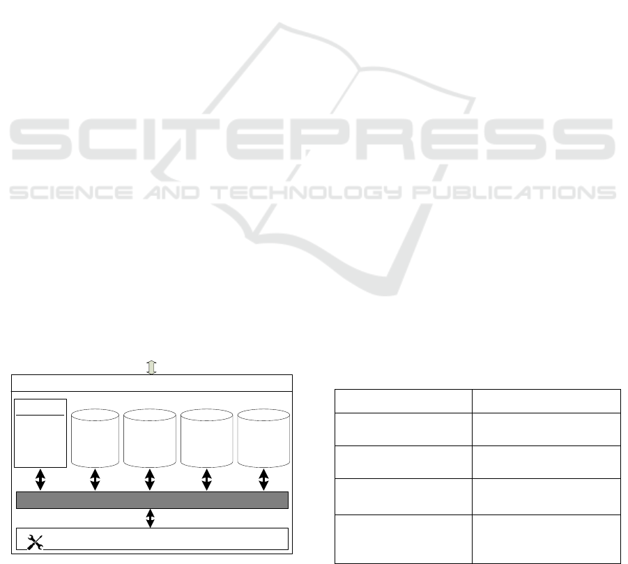
Figure 5: DGS Architecture.

Figure 5 shows the architecture of our DGS. A

decision maker, the user, uses a GUI to interact with

the system. The user provides inputs and then runs the

DGS Analytics Engine in Unity (Nachawati et al.,

2017), which translates the Analytical Model (AM)

code to low level code understood by an optimization

tool like the CPLEX solver and then executes it. The

user then receives an optimized release schedule and

the associated best BWP configuration, similar to

Table 2. The components of the AM mimic the

formalization hierarchy shown in Figure 3. Note that

the Unity Analytics Engine transparently connects the

AMs to the lower-level, external tools. In our case,

the Analytical Model is translated, by Unity, to

Mixed-Integer Linear Program (MILP) code.

The DGS is an integral part of the Release

Scheduling Methodology, which contains the

following key steps:

1. Gather the ReleaseScheduling parameters

2. Model the BWP

3. Gather the SoftwareDevelopment parameters

4. Setup the Decision Guidance System (DGS)

input data for the To-Be BWP configuration

5. Run the DGS to produce the optimal NPV for

the To-Be configuration

6. Setup the DGS input data for the As-Is BWP

configuration

7. Run the DGS to produce the NPV for the As-Is

configuration

8. Run the DGS to calculate the total NPV of the

savings

In the first step, we gather the ReleaseScheduling

parameters which include potential software features

that might enable savings in the BWP. Feature

dependencies are established, and their sizes are

estimated. For the example described in section 2, the

ReleaseScheduling parameters are shown in table 3.

Table 3: ReleaseScheduling.Parameters.

Parameter Value

(business features)

{BF1, BF2, BF2, BF4}

(technical features)

{TF1}

(dependency graph)

{(TF1, BF1), (BF1, BF2),

(TF1, BF3), (BF1, BF4)}

(feature size)

{(TF1,140), (BF1,140),

(BF2,280), (BF3,280),

(BF4,280)

ICEIS 2020 - 22nd International Conference on Enterprise Information Systems

392

Table 3: ReleaseScheduling.Parameters (cont.).

Parameter Value

(time horizon)

520

DiscountRate

(daily)

0.01923076923%

(number releases)

(release duration)

In step 2, the BWP is modelled. The top-level or

root process is defined; in our example we call it

‘Adj’. Each potential process alternative is defined

along with their inputs, outputs, labor rates and the

features that enable them. Each process is assigned a

type of atomic, AND or OR. The daily number of

inputs to the BWP, called Demand is set, and the days

when labor payments are made are determined. This

is important in order to account for the fact that an

amount of cash disbursed in the future is worth less

than the same amount of cash disbursed today. In our

example, we use the rate of 5% per year to discount

the labor payments. These parameters are assigned to

the formalization components BSN.parameters and

Service.parameters. For the example in Section 2, the

parameters are shown in Tables 4, 5, 6 and 7. Note

that the parameters in Table 4 are a numerical

codification of the BWP diagrams in Figures 1 and 2.

Table 4: BSN.Parameters.

Parameter Value

LR (Labor Roles) {IA, AO, A, S}

Rate

{(IA, 160), (AO, 400),

(A, 0), (S, 0)}

NLP (Number Labor

Payments)

LaborPayDay [60,120,180,240,520]

BSNI

(top-level process input)

{User Application}

BSNO

(top-level process output)

{}

Demand

(# top-level inputs)

100

ServicesSet

(space of alternatives)

{Adj, A, B, C, AA, AB,

AC, BA, BB, CA, CB}

rootID

(id of top-level process)

Adj

Table 5: Service.Parameters part 1.

id Type Input Output

Sub

services

RBF

Adj AND A, B, C

N/A

A OR AA,AB,AC

B OR BA, BB

C OR CA, CB

AA Atomic UA CA,NCN

N/A

AB Atomic UA CA,NCN BF1

AC Atomic UA CA,NCN BF4

BA Atomic CA AA

BB Atomic CA AA BF2

CA Atomic AA AL

CB Atomic AA AL BF3

Table 6: Service.Parameters part 2.

id Input Output

IO Thru

Ratio

AA UA CA 70%

AA UA NCN 30%

AB UA CA 70%

AB UA NCN 30%

AC UA CA 70%

AC UA NCN 30%

BA CA AA 100%

BB CA AA 100%

CA AA AL 100%

CB AA AL 100%

Table 7: Service.Parameters part 3.

id Role Input Output

RoleTime

PerIO

AA IO UA

0.250

AA IO CA 0.125

AA IO NCN 0.219

AB IO UA

0.145

AB S CA 0.000

AB S NCN 0.000

AC A UA

0.063

AC S CA 0.000

AC S NCN 0.000

BA AO CA

0.042

Decision Guidance on Software Feature Selection to Maximize the Beneﬁt to Organizational Processes

393

Table 7: Service.Parameters part 3 (cont.).

id Role Input Output

RoleTime

PerIO

BA AO

AA 0.208

BB AO CA

0.021

BB AO

AA 0.129

CA AO AA

0.021

CA AO

AL 0.167

CB AO AA

0.017

CB AO

AL 0.083

In step 3 of the methodology, we gather the

SoftwareDevelopment parameters as shown in

Table 8 for our example.

In step 4, we setup the DGS input data for the To-

Be configuration. All the parameters above are coded

in a JSON file which is used as input to the DGS.

In step 5, we run the DGS, which translates the

Analytical Model to Mixed-Integer Linear

Programming code and invokes the MILP solver to

produce the optimal NPV for the To-Be BWP

configuration. The main DecisionVariables, that are

instantiated during the optimization are IBF(r)

(Implemented Business Features), ITF(r)

(Implemented Technical Features) and On(id,r),

which indicates whether process id belongs to the best

BWP configuration for release r. The second column

in Table 2 captures the values of IBF and ITF for each

release r, while the third column shows the processes

that have On=1.

Table 8: SoftwareDevelopment.Parameters.

Parameter Value Unit

(Team Size)

(Dev Productivity)

1 (points/day)

(Dev Cost)

1,040 (US$/point)

(Operations Cost)

0.25 (US$/point/day)

(System Size prior

to development)

0 (points)

NSP

(# Soft Payments)

SWPayDay [60,120,180,240,520]

With the DecisionVariables instantiated, the daily

cost of the To-Be BWP and the software development

is calculated according to the Computation

formalization and shown in Table 9.

Note that the daily cost is accrued but only paid on

pay days and in our example, there are only 5

payments during the time horizon of 2 years, or 520

business days.

Table 9: To-Be Daily Cost.

Daily Cost

Rel BWP Software

1 $ 18,715.20 $ 5,200.00

2 $ 14,584.00 $ 5,275.00

3 $ 12,120.00 $ 5,350.00

4 $ 9,320.00 $ 5,425.00

After 4 $ 7,000.00 $ 300.00

Table 9 shows that the least costly BWP

configuration is the one after all releases are

implemented. This is expected because the

availability of all software features enables the best

BWP of all possible alternatives. Table 9 also shows

that after the software is implemented, there is a daily

labor cost to operate the software.

Once the daily cost is computed, the cash flow

disbursement is calculated for each day of the time

horizon. The NPV is the sum of the cash flows of the

BWP plus the software, discounted at 5% per year.

Table 10 shows the NPV results.

Table 10: NPV of the To-Be Configuration.

BWP

Cash Flow

Software

Cash Flow

NPV

1 -1,122,912.00 -312,000.00 -1,418,452.05

2 -875,040.00 -316,500.00 -1,164,360.35

3 -727,200.00 -321,000.00 -1,012,540.33

4 -559,200.00 -325,500.00 -844,799.39

after 4 -1,960,000.00 -84,000.00 -1,849,505.46

Accumulated NPV(To-Be): -6,289,657.59

Once the NPV of the To-Be is determined in step

5, in step 6, we setup the DGS input data in

preparation for the calculation of the NPV of the As-

Is. Basically, the decision variables are instantiated so

that the resulting BWP configuration is the one before

the system is developed, that is, AA, BA, CA, as

shown in the first row of Table 2.

ICEIS 2020 - 22nd International Conference on Enterprise Information Systems

394

In step 7, we run the DGS to produce the NPV for

the As-Is, which is shown in Table 11. Note that there

is no cost for software development.

In step 8, we run the DGS to calculate the total

NPV of the savings, which is the NPV of the To-Be

minus the NPV of the As-Is. The result is

2,796,271.21, which means that investing in the

software release schedule as depicted in Table 2,

reduces the total cost by almost 3 million US dollars

over 2 years.

Table 11: NPV of the A-Is Configuration.

Release BWP Cash Flow NPV

1 -1,048,051.20 -1,036,028.95

2 -1,048,051.20 -1,024,144.61

3 -1,048,051.20 -1,012,396.59

4 -1,048,051.20 -1,000,783.34

after 4 -5,539,699.20 -5,012,575.31

Accumulated

PV(As-Is): -9,085,928.80

5 CONCLUSION AND FUTURE

WORK

In this paper we introduced a software release

scheduling approach that is more precise than existing

value-based approaches because it is based on a

formal model of the Business Workflow Process and

its evolution following the implementation of

software features. We described the approach

intuitively, defined the formal model, explained the

Decision Guidance System and demonstrated the

methodology through an example.

There are many areas for future work, for

example, a case study can be conducted, and the

approach can be extended to include non-labor costs

such as office space and IT infrastructure.

REFERENCES

Boehm, B. W., & Sullivan, K. J. (2000). Software

economics: A roadmap. Proceedings of the Conference

on The Future of Software Engineering - ICSE ’00,

319–343.

Brodsky, A., Krishnamoorthy, M., Nachawati, M. O.,

Bernstein, W. Z., & Menascé, D. A. (2017).

Manufacturing and contract service networks:

Composition, optimization and tradeoff analysis based

on a reusable repository of performance models. 2017

IEEE International Conference on Big Data (Big

Data), 1716–1725.

Brodsky, Alexander, & Luo, J. (2015). Decision Guidance

Analytics Language (DGAL)-Toward Reusable

Knowledge Base Centric Modeling. 17th International

Conference on Enterprise Information Systems

(ICEIS), 67–78.

Cleland-Huang, J., & Denne, M. (2005). Financially

informed requirements prioritization. Proceedings.

27th International Conference on Software

Engineering, 2005. ICSE 2005., 710–

Denne, M., & Cleland-Huang, J. (2004). The incremental

funding method: Data-driven software development.

IEEE Software, 21(3), 39–47.

Denne, Mark, & Cleland-Huang, J. (2003). Software by

Numbers: Low-Risk, High-Return Development.

Prentice Hall.

Devaraj, S., & Kohli, R. (2002). The IT Payoff: Measuring

the Business Value of Information Technology

Investments. FT Press.

Elsaid, A. H., Salem, R. K., & Abdelkader, H. M. (2019).

Proposed framework for planning software releases

using fuzzy rule-based system. IET Software, 13(6),

543–554.

Hannay, J. E., Benestad, H. C., & Strand, K. (2017). Benefit

Points: The Best Part of the Story. IEEE Software,

34(3), 73–85.

Maurice, S., Ruhe, G., Saliu, O., & Ngo-The, A. (2006).

Decision Support for Value-Based Software Release

Planning. In Value-Based Software Engineering (pp.

247–261). Springer, Berlin, Heidelberg.

Nachawati, M. O., Brodsky, A., & Luo, J. (2016). Unity: A

NoSQL-based Platform for Building Decision

Guidance Systems from Reusable Analytics Models.

Technical Report GMU-CS-TR-2016-4. George Mason

University.

Nachawati, M. O., Brodsky, A., & Luo, J. (2017). Unity

Decision Guidance Management System: Analytics

Engine and Reusable Model Repository. ICEIS (1),

312–323.

Pucciarelli, J., & Wiklund, D. (2009). Improving IT Project

Outcomes by Systematically Managing and Hedging

Risk. IDC Report.

Riegel, N., & Doerr, J. (2014). An Analysis of Priority-

Based Decision Heuristics for Optimizing Elicitation

Efficiency. In Requirements Engineering: Foundation

for Software Quality (pp. 268–284). Springer

International Publishing.

The Standish Group. (2014). CHAOS Manifesto 2014

Van den Akker, M., Brinkkemper, S., Diepen, G., &

Versendaal, J. (2005). Determination of the Next

Release of a Software Product: An Approach using

Integer Linear Programming. CAiSE Short Paper

Proceedings.

Decision Guidance on Software Feature Selection to Maximize the Beneﬁt to Organizational Processes

395