A Least Squares based Groupwise Image Registration Technique

Nefeli Lamprinou, Nikolaos Nikolikos and Emmanouil Z. Psarakis

Computer Engineering and Informatics Department, Patras, Greece

Keywords:

Groupwise Registration, Congealign, Image Alignment, Medical Imaging, Multi-modal Alignment,

Self Quotient Image.

Abstract:

Compared with pairwise registration, groupwise registration is capable of handling a large-scale population

of images simultaneously in an unbiased way. In this work we improve upon the state-of-the-art pixel-level,

Least-Squares (LS) based groupwise image registration methods. Speciﬁcally, we propose a new iterative

algorithm which outperforms in terms of its computational cost, a recently introduced LS based iterative

congealing scheme. Namely, the particle system that was introduced in that work is used and by imposing its

“center of mass” to be motionless, during each iteration of the minimization process, a sequence of “centroid”

images whose limit is the unknown “mean” image is optimally in closed form deﬁned, thus solving in a

reduced computational cost the groupwise problem. Moreover, the registration technique is properly adapted

by the use of Self Quotient Images (SQI) in order to become capable for solving the groupwise registration of

multimodal images. Since the proposed congealing technique is invariant to the size of the image set, it can be

used for the successful solution of the problem on large image sets with low complexity. From the application

of the proposed technique on a series of experiments for the groupwise registration of face, unimodal and

multimodal magnetic resonance image sets its performance seems to be very good.

1 INTRODUCTION

The problem of image congealing or groupwise align-

ment/registration is an important one within the com-

puter vision community. A good congealing algo-

rithm can be used as preprocessing to notably improve

the performance of other vision tasks within differ-

ent research areas (Liu and Wang, 2014). Compared

to the pairwise registration, groupwise registration is

capable of handling a large-scale population of im-

ages simultaneously in an unbiased way. Speciﬁcally,

it eliminates the requirement of choosing a reference

image, thus avoiding a registration bias. Our work

improves upon the most widely recognized area based

LS based state-of-the-art approach. Most area based

state-of-the-art algorithms can be considered (Niko-

likos et al., 2017) as variations of a common base

framework. The basic idea is to use one image at

a time as the held out image and the rest of the en-

semble as the stack. Having done that the goal is

to minimize, in an iterative fashion, an error func-

tion deﬁned over all of the ensemble, by estimating a

warp update for the held out image that aligns it with

the stack. Algorithms based on the aforementioned

https://orcid.org/0000-0002-9627-0640

idea include groupwise methods with entropy based

cost functions, such as the algorithms proposed in

(Learned-Miller, 2006), (Zollei, 2006),(Vedaldi and

Soatto, 2006) as well as with LS based cost func-

tions such as the methods proposed in (Cox et al.,

2008),(Cox et al., 2009),(Cox, 2010),(Xue and Liu,

2012). In (Storer and Urschler, 2010) an error func-

tion based on mutual information that copes with pos-

sible variations in appearance between similar objects

of the same class is deﬁned. In addition, in (Huang

et al., 2007) and (Huang et al., 2012) extended en-

tropy based congealing for the usage on real world

complex images is proposed. Recently, in (Huizinga

et al., 2016),(Guyader et al., 2018) groupwise regis-

tration techniques were tailored for the registration of

quantitative MRI datasets. LS based congealing al-

gorithms tend to perform better in terms of conver-

gence rate and accuracy. In the LS case, there are two

ways to align the held out image with the stack using

gradient descend optimization techniques. The ﬁrst

one, which is known as the forward LS congealing

approach has poor alignment performance, especially

for strong initial misalignments, but has a really low

computational cost. On the other hand the inverse LS

congealing approach that computes a common warp

120

Lamprinou, N., Nikolikos, N. and Psarakis, E.

A Least Squares based Groupwise Image Registration Technique.

DOI: 10.5220/0009180701200127

In Proceedings of the 15th International Joint Conference on Computer Vision, Imaging and Computer Graphics Theory and Applications (VISIGRAPP 2020) - Volume 4: VISAPP, pages

120-127

ISBN: 978-989-758-402-2; ISSN: 2184-4321

update for all images of the stack by utilizing the in-

verse approach presented in (Cox et al., 2008) out-

performs the forward LS in both accuracy and robust-

ness, but its high computational cost, due to existing

nested loops, makes its use prohibitive for large image

sets as the number of sub-problems grows quadrati-

cally with respect to the image set’s size. Moreover,

additional robustiﬁcation is needed in order to be able

to handle outliers (Cox, 2010).

The proposed groupwise method improves upon

all the desirable characteristics of the state-of-the-art

inverse method, while maintaining a linear to the set

size computational cost, similar to that of the forward

approach. Moreover, the proposed technique is com-

putationally cheaper than its predecessor (Nikolikos

et al., 2017) where, in each iteration of the algorithm,

the singular value decomposition of the pseudo in-

verse of the Jacobian matrices over the entire ensem-

ble of the images was needed. Finally, the proposed

technique, as well as its predecessor, can be easily

adapted to make use of feature descriptors, instead of

intensity values, as the representation of each image,

as the majority of the unsupervised intensity-based

techniques during the joint alignment process do, in

order to cope with background variations.

The remainder of this paper is organized as fol-

lows: In Section 2, we formulate the image congeal-

ing problem and several issues related with it are ex-

amined. In Section 3, the particle system that was in-

troduced in (Nikolikos et al., 2017) that is strongly re-

lated to the geometric transformations of the image’s

set is reviewed, and the proposed optimal deﬁnition

of the ”centroid” image is presented. In Section 4,

the results of the experiments we have conducted are

presented. Finally, Section 5 concludes our paper.

2 PROBLEM FORMULATION

2.1 Preliminaries

Let us consider a set containing N images:

= {i

}

n=1

(1)

that belong to the same cluster, that is S

contains a

group of similar in shape and aligned images, where

i denotes the column-wise of length N

vectorized

version of size N

×N

image I. Then, it is well known

that the “mean” image which is deﬁned by:

∑

n=1

(2)

constitutes the most representative image for the clus-

ter and it can result from the solution of the following

optimization problem:

= arg min

i ∈ R

{

∑

n=1

i − i

} (3)

where ||x||

denotes the l

norm of vector x.

Let us now consider, apart from the set S

, the follow-

ing set:

(P) = {i

)}

n=1

(4)

containing the geometrically distorted vectorized im-

ages of set S

of (1) where

P = {p

}

n=1

, (5)

is a set of N warp parameter vectors. Under the used

warping transformation w( . ; p

)

, which is param-

eterized by the vector p

∈ R

, each pixel x of the

Region of Interest of image i

of set S

is mapped onto

the pixel

x of the corresponding image i

) of set

(P), i.e.:

(

x; p

) = I

(w(x; p

)). (6)

In other words the set S

(P) is generated by the

following process:

w(.;p

)

−−−−→ i

)

w(.;p

)

−−−−→ i

)

w(.;p

)

−−−−→ i

)











≡ S

(P) (7)

where, as it was already mentioned, all images belong

to the same cluster, are aligned and the “mean” image

is deﬁned by (2).

Then, congealing, or groupwise registration (Liu

and Wang, 2014) can be deﬁned as the minimization

problem of a misalignment function, let us denote it

by E (P), which is calculated over the set S

(P), for

a warping function that models the parametric form

of the misalignment to be removed. In general, solv-

ing the image congealing problem is not an easy task

and its complexity heavily depends on several factors,

such as the size of the ensemble and the strongness of

the geometric distortions, to name a few.

Although, in some cases the aforementioned prob-

lem can be easily solved (Nikolikos et al., 2017), in

the general case, its solution results in a highly nonlin-

ear and computationally demanding procedure. This

is basically because the goal of estimating the collec-

tion of the unknown parameters should be achieved

by deﬁning a misalignment function E (P) over the

entire ensemble of images. Such a function, which is

In this paper, to model the warping process we are go-

ing to use the class of afﬁne transformations with p

∈ R

A Least Squares based Groupwise Image Registration Technique

121

known as the Cumulative Squared Misalignment Er-

ror (CSME):

E (P) =

∑

n=1

ε(p

) (8)

where

ε(p

) =

∑

m=1,m6=n

||i

) − i

)||

, (9)

has all these characteristics and was proposed in (Cox

et al., 2008). However, since the above total cost func-

tion is difﬁcult to be optimized directly (Tong et al.,

2009), the iterative minimization of the individual

cost function ε(p

) for each geometrically distorted

image i

), given an initial estimation of the warp-

ing parameter p

, m = 1,2,··· , N, was proposed.

In general, aligning each image of the aforemen-

tioned set with a stack of images, results in a problem

which is heavily depended on the initial conditions

of the average image. This is obvious since indepen-

dently of the blurriness of the basis images, the aver-

age image before the alignment of images is blurred.

Thus, using the average image to control the direction

of the corrections of the parameters, with all the ﬁne

details of the image lost, the algorithm is at the mercy

of the initial conditions (Cox et al., 2008). In order to

avoid this undesired effect, LS congealing avoids us-

ing the mean image and for improving the quality of

the alignment an inverse compositional LS congeal-

ing algorithm was proposed.

However, in the next section we are going to ex-

plore ways of obtaining the alignment of the ensemble

in (4) without having to align all the individual pairs

resulting from it. Instead, we are going to align each

image with the “mean” image, which we are going

to relate with the “centre of mass” of the geometric

transformations set (5).

2.2 A Simpliﬁed Misalignment Function

In (Nikolikos et al., 2017) the following total mean

misalignment function:

(P;

) =

∑

n=1

− i

)||

(10)

where

denotes the unknown “mean” image, was

proposed. It is clear that the above proposed mis-

alignment function is separable, but is a non linear

function of each member of the set of warp parame-

ters deﬁned in (5). Thus, for each one of the cost func-

tions involved into (10) its minimization requires non-

linear optimization techniques either by using direct

search or by following gradient-based approaches. As

is customary in iterative techniques, the original opti-

mization problem is replaced by a sequence of sec-

ondary optimizations. Each secondary optimization

relies on the outcome of its predecessor, thus gener-

ating a chain of parameter estimates which hopefully

converges to the desired optimizing vector. At each it-

eration, we do not have to optimize the objective func-

tion but an approximation to this function. Assum-

ing that at the k-th iteration of the iterative procedure

(k) is ”close” to some nominal parameter vector

then we write p

(k) =

+∆p

(k), where ∆p

(k) de-

notes a vector of perturbations. We recall here that in

order to be able to compute the optimal perturbations

∆p

(k), the nominal parameter vector

as well as

the “mean” image

must be known. By assigning to

the nominal parameter vector

the estimation of the

previous iteration, i.e.: p

(k − 1) →

, the optimal

perturbations can be computed as follows:

∆p

(k) = A

(k − 1))(

− i

(k − 1))) (11)

where

(

(k − 1)) =

(

(k − 1))

(

(k − 1)))

−1

(

(k − 1))

(12)

is the M × N

pseudo inverse of the Jacobian ma-

trix G

(

(k − 1)) evaluated at

(k − 1), (Baker and

Matthews, 2004).

Note however, that since the “mean” image

unknown the optimal values of the perturbations in

(11) can not be computed. Moreover, the use of the

following average of the warped vectorized images:

(k) =

∑

n=1

(k − 1)) (13)

leading to a similar approach with the forward one,

will have a poor alignment performance (Cox, 2010).

In order to overcome this obstacle, in (Nikolikos et al.,

2017) a particle system was deﬁned and the motion of

each particle was explicitly related with the estimated

values of a corresponding parameter vector during the

iterative procedure of the optimization. We are going

to review this particle system and use it to optimally

deﬁne, through a new optimization problem the “cen-

troid” vectorized image.

2.3 The Particle System

Let us consider that each member of set S

(P) de-

notes the starting position of a particle of mass m =

1/N that can be moved into R

. Hence the set S

(P)

could be considered as a set containing the starting

positions of a system of N isobaric particles. Let

(k) be the position of the n-th patricle at the k-th

VISAPP 2020 - 15th International Conference on Computer Vision Theory and Applications

122

instant as it moves into R

. Then, its trajectory can

be deﬁned with the following position’s set:

= {p

(k), k = 0, 1, 2, · · · }, (14)

with its ﬁrst and last element p

(0), lim

k→∞

(k) denot-

ing its starting and ending position respectively and

its motion, can be easily expressed by the following

simple motion model:

(k) = p

(k − 1) + ∆p

(k), k = 1, 2, ··· , (15)

with the vector ∆p

(k) denoting its differential move-

ment.

The position of the center of mass of the whole

particle system, at the k-th instant:

p(k) =

∑

n=1

(k) (16)

can be used as the origin of the moving coordinate

system. Speciﬁcally, the position of the n-th particle

at the k−th instant with respect to the new origin

p(k)

can be expressed as follows:

(k) =

p(k) + q

(k), k = 1, 2, ··· . (17)

Note that the vectors q

(k), n = 1, 2,··· , N denote

the positions of the particles in the new coordinate

system and are zero mean, that is:

∑

n=1

(k) = 0. (18)

As the optimization (time) goes on, the position vec-

tors of the particles change with time and thus, in gen-

eral, the center of mass moves too with its velocity

given by:

∆

p(k) =

p(k) −

p(k − 1) =

∑

n=1

∆p

(k) (19)

where

p(k),

p(k − 1), k = 1, 2, ··· are the center of

mass of the N− sized particle system at two consecu-

tive instances. Then, according to Proposition 3.1 in

(Nikolikos et al., 2017), the mean geometric transfor-

mation remains the same over the iteration process,

i.e.:

p =

p(k), k = 0, 1,··· (20)

if the total momentum of the particle system is zero,

that is:

∆

p(k) = 0. (21)

This transformation totally speciﬁes the geometric de-

formation of the ”mean” image and we are going to

use it in the next section for deﬁning the ”centroid”

image.

2.4 The “Centroid” Image

To this end, let us deﬁne a sequence of vectorized im-

ages:

= {i(k)}

∞

k=1

, (22)

having the following two properties (Nikolikos et al.,

2017):

• P

: The k−th member of the sequence, is the

”centroid” image of the corresponding iteration of

the minimization process

• P

: The limit of the sequence is the unknown

”mean” image, that is:

lim

k→∞

i(k) =

, (23)

and the following average quantities:

A(k) =

∑

n=1

(k − 1)) (24)

b(k) =

∑

n=1

(k − 1))i

(k − 1)) (25)

∆p(k) =

∑

n=1

∆p

(k). (26)

As it is clear from (26),

∆p(k) is the average of the

optimal geometric perturbations at the k−th iteration

of the minimization process. Note also that this av-

erage coincides with the velocity ∆

p(k) of the centre

of mass of the particle system deﬁned in (19). By ex-

ploiting this fact, in the following we deﬁne a mean-

ingful optimization problem and use it for optimally

deﬁne the “centroid” image.

To this end, let P

k−1

be the set P deﬁned in (5)

containing the values of the parameter vectors result-

ing after the k − 1-th iteration of the minimization

of the non-linear cost function E

k−1

;i(k − 1)) de-

ﬁned in (10). Then, for the optimal deﬁnition of the

“centroid” image we can deﬁne the following con-

strained optimization problem:

min

i(k)

k−1

;i(k))

subject to: A(k)i(k) = b(k).

(27)

As we are going to see in the next theorem, the

solution of the aforementioned problem differentiates

the “centroid” image from the “mean” one for each

ﬁnite value of k while it tends to the “mean” as k → ∞,

thus ensuring that property P

in (23) holds.

Theorem 2.1. The optimal solution of the optimiza-

tion problem (27) is given by:

i(k) = (I − A

†

(k)A(k))i

(k) + A

†

(k)b(k) (28)

A Least Squares based Groupwise Image Registration Technique

123

where I is the identity matrix of size N

× N

†

(k) the pseudo inverse of matrix A(k) deﬁned in Eq.

(24) and b(k) the vector deﬁned in Eq. (25) respec-

tively.

Proof. The proof is easy and is left to the reader.

Note that in each iteration the optimal “centroid”

image is the superposition of two components with

each one being associated with an appropriate sub-

space of the space R

of the vectorized images.

It can be easily proved that the ﬁrst component co-

incides with the component i

(k) while the second

one with the component i

(k) as they were deﬁned

in (Nikolikos et al., 2017). However, we must stress

at this point that its computational cost is very low

as it compared with the solution proposed in (Niko-

likos et al., 2017) where, in each iteration, the Sin-

gular Value Decomposition of matrix A(k) was nec-

essary. Note also that the second component of the

“centroid” image ensures that the Condition (21) is

satisﬁed.

An outline of the proposed algorithm follows.

Input: Image set S

(P), the vector

p and the

ROI

Set k = 1

repeat

for n = 1 : N do

Compute the Jacobian of the image

(k − 1))

end

Use (13, 24, 25) to update

(k), A(k) and

b(k)

Use Eq. (28) to compute the “centroid”

i(k);

for n = 1 : N do

Use (11) to compute the optimal

perturbations ∆p

(k) that align

image i

(k − 1)) to the

“centroid” image i(k) and warp the

image accordingly

end

k = k + 1

until E

k−1

;i(k)) has converged;

Output: Image set S

Algorithm 1: Outline of the Proposed LS-Centroid

Congealing Algorithm.

3 REGISTRATION OF

MULTI-CONTRAST MR

IMAGES

In this section we are going to present the most com-

mon different modalities of MR Images. Then, the

edge preserving ﬁltering scheme, originally proposed

in (Nikolikos et al., 2019), for their preprocessing will

be shortly explained.

3.1 Multi-contrast MR Images

Unlike imaging using radiation, in which the contrast

depends on the different attenuation of the structures

being imaged, the contrast in MR Images depends on

the magnetic properties and the number of hydrogen

nuclei existing in the area being imaged. The two ba-

sic types of MR Images, often referred to as T 1 and

T 2 images, are T 1-weighted and T 2-weighted im-

ages. The main difference between those types of MR

Images is the timing of the radiofrequency pulse se-

quences that is used to make them. The timing pulse

sequence used for T 1 images results in images which

highlight fat tissue, while the timing pulse sequence

used for making T 2 images results in images which

highlight fat, as well as, water within the body. Un-

like T 1 and T 2 images, Proton Density (PD) images

do not display the magnetic characteristics of the hy-

drogen nuclei, but the number of nuclei in the area

being imaged. Finally, magnetic resonance angiogra-

phy (MRA) is a type of MRI that looks speciﬁcally at

the body’s blood vessels.

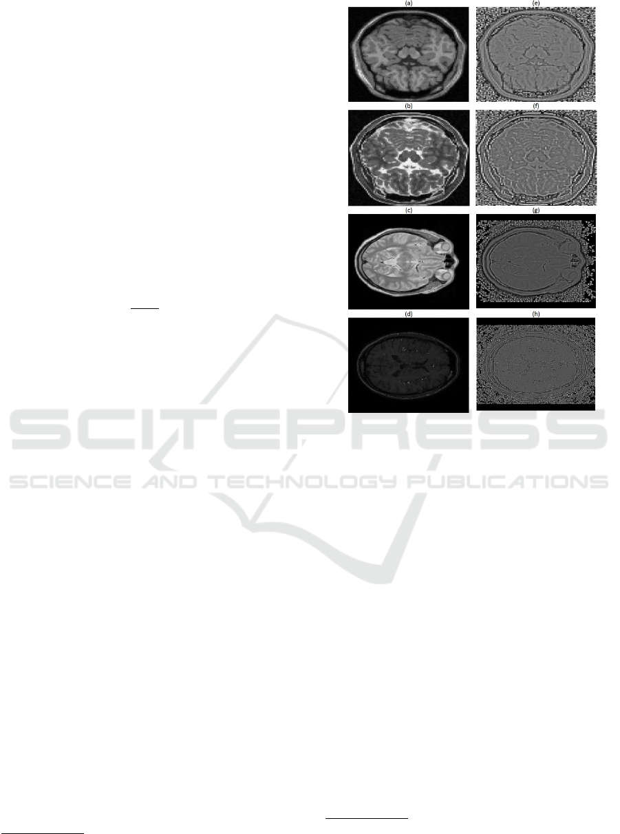
In Figure 1 four slices, one for each aforemen-

tioned MRI type of images, are shown. It is clear that

the different types of MRI images have totally dif-

ferent intensity distributions, a fact that has the same

impact as the strong photometric distortions. Thus,

the use of intensity based techniques for aligning, ei-

ther pairwise or groupwise, multi-modal images does

not constitute a good choice for the solution of the

problem at hand. In order to be able to use such area

based techniques, the preprocessing of the images or

volumes with a known edge preserving ﬁlter was pro-

posed (Nikolikos et al., 2019).

3.2 Self Quotient Images

A powerful image processing based technique achiev-

ing invariance to local illumination distortions was

proposed in (Wang et al., 2004) that results, in the

transformation of the image, to the well known SQI.

According to this technique, the SQI is deﬁned as

the ratio of a given image to its smoothed version

VISAPP 2020 - 15th International Conference on Computer Vision Theory and Applications

124

and aims to construct a shadow invariant represen-

tation of the original image. SQI is deﬁned as the

ratio of a given image to its smoothed version aim-

ing to construct a brightness invariant representation

of the initial image. Note that the invariance of that

image’s representation holds for all contrast types of

MR images and volumes, since for both brighted and

no-brighted tissues the ratio effectively removes the

brightness effects. To this end, let I

(x) be a smoothed

version of the image I(x) that results from its convo-

lution with the isotropic Gaussian kernel G

(x), with

the subscript denoting its standard deviation. That is:

(x) = I(x) ∗ G

(x) (29)

where “∗” denotes the 2-D convolutional operator.

Suppose also that we are given a set of coordinates

x within the image, which consists the target area or

target. Then, the Self Quotient Image is deﬁned as

follows:

Q(x) =

I(x)

(x)

,∀x ∈ T. (30)

Note that the deviation of the Gaussian kernel con-

trols the width of the edges in the image deﬁned in

Eq. (30). To address the noise as well as the out-

liers problem from which SQI suffers from we use

a hard thresholding procedure. Considering pairwise

registration, let σ

,σ

be the standard deviations of

the vectorized counterparts of SQIs Q

(.) and Q

(.),

where Q

(.) and Q

(.) the template and the warped

image respectively. Then, we can deﬁne the follow-

ing threshold:

= µ min{σ

,σ

} (31)

with 0 < µ < 1 a parameter that can be used to have

additional control over the value of threshold T

. In all

experiments we have conducted we set µ = 1/2. The

SQIs resulting from the application of the above men-

tioned procedure on the four different contrast type

MRI slices that are shown in Figure 1. In the context

of the group-wise problem, we calculate the threshold

for each pair that consists of an image of the ensem-

ble and the current centroid image. Having ﬁltered

out the strong photometric distortions, we can use the

above mentioned area based technique for solving the

groupwise alignment problem.

4 EXPERIMENTS

In this section we are going to present our results by

applying the proposed technique in a series of exper-

iments on real as well as artiﬁcial data. The ﬁrst ex-

periment is conducted with data from AR database

http://www2.ece.ohio-state.edu/aleix/ARdatabase.

html

Figure 1: (a)-(d): Original T 1, T 2, PD and MRA images

respectively, (e)-(h): The corresponding SQI’s after thresh-

olding for T 1, T 2, PD and MRA images respectively.

The rest of the experiments are conducted with artiﬁ-

cial MRI data obtained from Brainweb Database

and

real data from IXI Dataset

, to test the alignment of

images of the same or different modalities. In two ex-

periments we also applied artiﬁcial warps to the im-

ages. In order to control the strongness of the used

warps applied to the initial images, the framework

presented in (Baker and Matthews, 2004) was used,

with the distortion parameter σ taking various values.

4.1 AR Experiment

Since the groupwise alignment solution proposed de-

rives from the one proposed in (Nikolikos et al.,

2017), in this experiment we replicated the experi-

ment conducted using geometrically distorted images

from AR database, with the distortion parameter σ

taking values in the interval [1,10] with the values 1

and 10 corresponding to the smallest and strongest ge-

ometric distortions respectively. The resulting mean

images conﬁrm that the two techniques have the same

https://www.mcgill.ca/bic/software/brainweb-mri-

simulator

https://brain-development.org/ixi-dataset/

A Least Squares based Groupwise Image Registration Technique

125

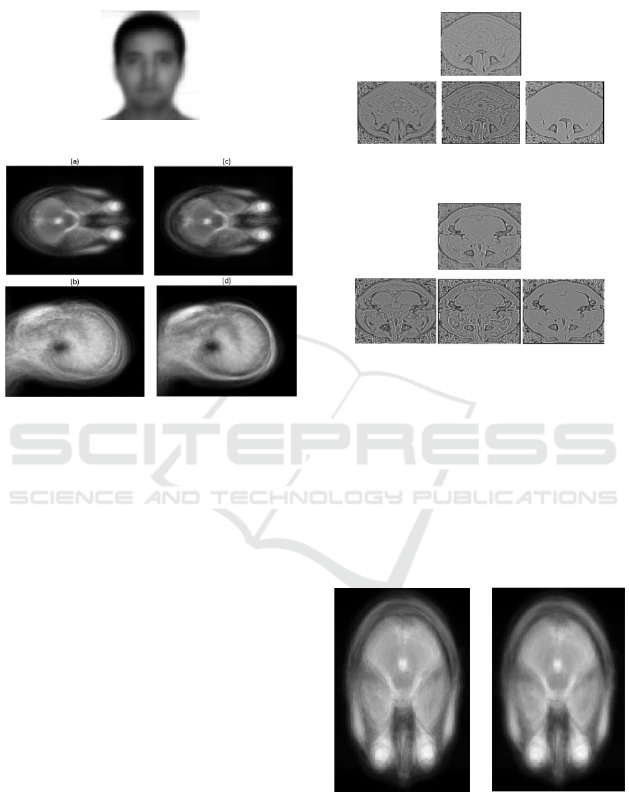
Figure 2: Mean image of 50 images with σ = 4 after align-

ment.

Figure 3: (a): Original mean image of 50 T 2 images, (b):

Original mean image of 50 T 1 images, (c): Mean image of

(a) after alignment, (d): Mean image of (b) after alignment.

performance, as we may see in Figure 2, although the

proposed closed form solution ensures that the latter

is much faster than its predecessor.

4.2 MRI Experiments

We conducted a series of experiments with different

MRI image modalities, namely T1, T 2, PD and MRA.

4.2.1 Unimodal Alignment

First, we aim to align images from IXI Dataset con-

taining the same slice, of the same modality, from 50

different subjects. In Figure 3 we can see the mean

image in T 1 and T 2 cases.

It is obvious in Figure 3 that the contour of the

mean image after alignment is much clearer and more

deﬁned.

4.2.2 Multimodal Alignment in Artiﬁcial Data

In this experiment we align images from Brainweb

Database, where we add small artiﬁcial warps of σ =

1, aligning then across the same slice different modal-

ities T 1, T 2 and PD. In Figures 4 and 5 we see the

mean image for random slices, as well as the three

aligned images in each case.

Figure 4: Middle Top Image: Mean quotient image of three

below images after alignment, Bottom Row: T 1, T 2 and

PD quotient images respectively.

Figure 5: Middle Top Image: Mean quotient image of three

below images after alignment, Bottom Row: T 1, T 2 and

PD quotient images respectively.

4.2.3 Multimodal Alignment in Real Data

In this experiment we align images from IXI Dataset,

aligning them across the same slice different modali-

ties T 2, MRA and PD. In Figure 6 we see the mean

image for random slices from 28 subjects from each

modality, while in Figure 7 we can see an example

image from each modality, T 2, PD, MRA along with

their respective quotient images which are obviously

the ones that allow multi-modal registration.

Figure 6: Left Image: Original “mean” image of T 2 , MRA

and PD images, Right Image: “mean” image after align-

ment.

VISAPP 2020 - 15th International Conference on Computer Vision Theory and Applications

126

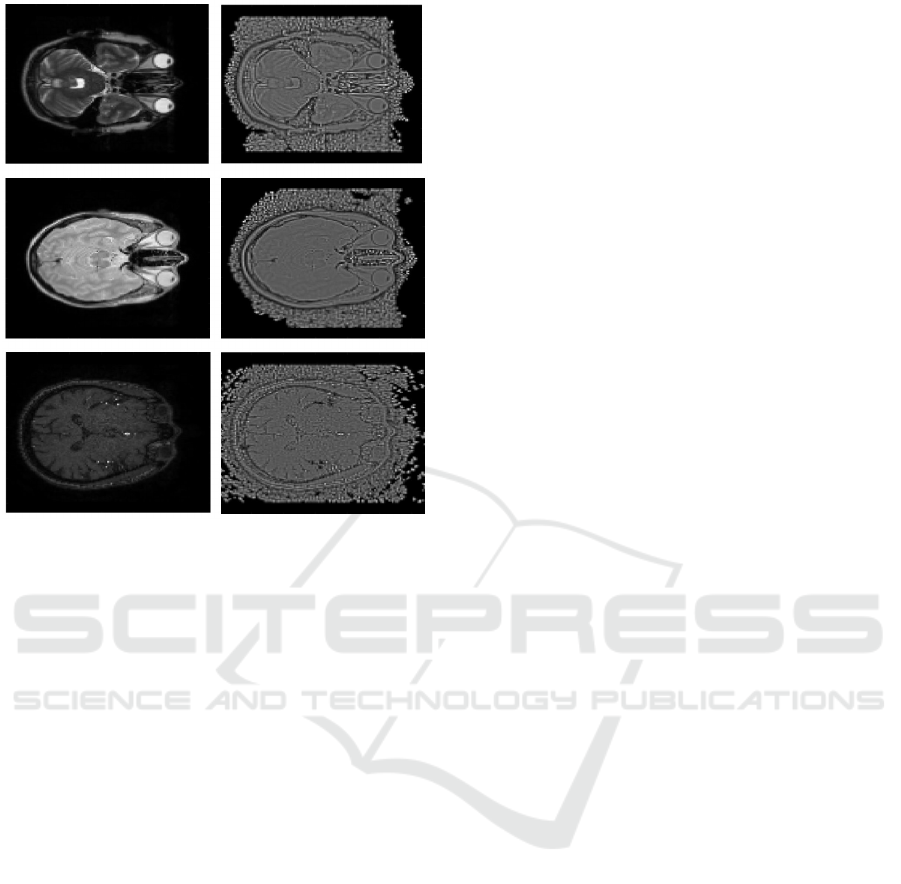
Figure 7: Top Row: T 2 image(left) and the respective quo-

tient image(right), Middle Row: PD image(left) and the

respective quotient image(right), Bottom Row: MRA im-

age(left) and the respective quotient image(right).

5 CONCLUSIONS

In this work a recently introduced Least-Squares

based groupwise image registration method was im-

proved in terms of its computational cost. This was

achieved by optimally deﬁning a sequence of “cen-

troid” images whose limit was the desired but un-

known “mean” image for solving the groupwise prob-

lem. In addition, the proposed technique was prop-

erly adapted for its use in the groupwise registration

of multimodal images. The performance of the pro-

posed technique, from its application on a number

of experiments, was very good. The extensive eval-

uation of its performance against other state of the

art groupwise registration techniques and its exten-

sion for solving the corresponding groupwise volume

problem are currently under investigation.

ACKNOWLEDGEMENTS

This research is implemented through the Operational

Program ”Human Resources Development, Educa-

tion and Lifelong Learning” and is co-ﬁnanced by the

European Union (European Social Fund) and Greek

national funds.

REFERENCES

Baker, S. and Matthews, I. (2004). Lucas-kanade 20 years

on: A unifying framework. International Journal of

Computer Vision 56(3), 221–255.

Cox, M. (2010). Unsupervised alignment of thousands of

images. PhD thesis, Queensland University of Tech-

nology, Brisbane, Queensland.

Cox, M., Sridharan, S., Lucey, S., and Cohn, J. (2008).

Least squares congealign for unsupervised alignment

of images. CVPR.

Cox, M., Sridharan, S., Lucey, S., and Cohn, J. (2009).

Least squares congealign for large number of images.

CVPR.

Guyader, Jean-Marie, Huizinga, Wyke, Poot, J., D. H., van

Kranenburg, Matthijs, Uitterdijk, A., Niessen, W. J.,

and Klein, S. (2018). Groupwise image registration

based on a total correlation dissimilarity measure for

quantitative mri and dynamic imaging data. Scientiﬁc

Reports, 8(1):13112.

Huang, G., Jain, V., and Learned-Miller, E. (2007). Unsu-

pervised joint alignment of complex images. In ICCV-

2007.

Huang, G. B., Mattar, M.and Lee, H., and Learned-Miller,

E. (2012). Learning to align from scratch. In Neural

Information Processing Systems.

Huizinga, W., Poot, D. H. J., Guyader, J.-M., Klaassen,

R., Coolen, B. F., van Kranenburg, M., van Geuns,

R. J. M., Uitterdijk, A., Polﬂiet, M., and et al., J. V.

(2016). Pca-based groupwise image registration for

quantitative mri. Med Image Anal., pages 65–78.

Learned-Miller, E. (2006). Data driven image models

through continuous joint alignment. IEEE T-PAMI,

28(2):236–250.

Liu, Q. and Wang, Q. (2014). Groupwise registra-

tion of brain magnetic resonance images: A review.

Journal of Shanghai Jiaotong University (Science),

19(6):755–762.

Nikolikos, N., Lamprinou, N., Boile, A., and Psarakis, E.

(2019). Multi-contrast mri volume alignment via ecc

maximization. In BioInformatics and BioEngineering

(BIBE). IEEE.

Nikolikos, N., Psarakis, E., and Lamprinou, N. (2017). A

new least squares based congealing technique. Else-

vier Pattern Recognition Letters, 95:58–64.

Storer, M. and Urschler, M. (2010). Intensity-based con-

gealing for unsupervised joint image alignment. In

ICPR, 2010.

Tong, C., Liu, X., Willer, F., and Tu, P. (2009). Automatic

facial landmark labelin with minimal supervision. In

CVPR, 2009.

Vedaldi, A. and Soatto, S. (2006). A complexity-distortion

approach to joint pattern alignment. In NIPS.

Wang, H., Li, S. Z., Wang, Y., and jun Zhang, J. (2004). Self

quotient image for face recognition. In International

Conference on Image Processing (ICIP), pages 1397–

1400. IEEE.

Xue, Y. and Liu, X. (2012). Image congealign via efﬁcient

feature selection. Applications of Computer Vision

(WACV).

Zollei, L. (2006). A Uniﬁed Information Theoretic Frame-

work for Pair- and Group-wise Registration of Medi-

cal Images. PhD thesis, MIT Computer Science and

Artiﬁcial Intelligence Laboratory.

A Least Squares based Groupwise Image Registration Technique

127