
Sentiment Analysis from Sound Spectrograms via Soft BoVW
and Temporal Structure Modelling
George Pikramenos
1,4
, Georgios Smyrnis
2
, Ioannis Vernikos
3,4
, Thomas Konidaris
4
,
Evaggelos Spyrou
3,4
and Stavros Perantonis
4
1
Department of Informatics & Telecommunications, National Kapodistrian University of Athens, Athens, Greece
2
School of Electrical & Computer Engineering, National Technical University of Athens, Athens, Greece
3
Department of Computer Science and Telecommunications, University of Thessaly, Lamia, Greece
4
Institute of Informatics & Telecommunications, NSCR-“Demokritos”, Athens, Greece
Keywords:
Sentiment Analysis, Speech Analysis, Bag-of-Visual-Words.
Abstract:
Monitoring and analysis of human sentiments is currently one of the hottest research topics in the field of
human-computer interaction, having many applications. However, in order to become practical in daily life,
sentiment recognition techniques should analyze data collected in an unobtrusive way. For this reason, ana-
lyzing audio signals of human speech (as opposed to say biometrics) is considered key to potential emotion
recognition systems. In this work, we expand upon previous efforts to analyze speech signals using computer
vision techniques on their spectrograms. In particular, we utilize ORB descriptors on keypoints distributed
on a regular grid over the spectrogram to obtain an intermediate representation. Firstly, a technique similar to
Bag-of-Visual-Words (BoVW) is used, where a visual vocabulary is created by clustering keypoint descriptors,
but instead a soft candidacy score is used to construct the histogram descriptors of the signal. Furthermore,
a technique which takes into account the temporal structure of the spectrograms is examined, allowing for
effective model regularization. Both of these techniques are evaluated in several popular emotion recognition
datasets, with results indicating an improvement over the simple BoVW method.
1 INTRODUCTION
The recognition of human emotional states consti-
tutes one of the most recent trends in the broader re-
search area of human computer interaction (Cowie
et al., 2001). Several modalities are typically used
towards this goal; information is extracted by sen-
sors, either placed on the subject’s body or within
the user’s environment. In the first case, one may
use e.g., physiological and/or inertial sensors, while
on the latter case cameras and/or microphones. Even
though video is becoming the main public means of
self-expression (Poria et al., 2016), people still con-
sider cameras to be more invasive than microphones
(Zeng et al., 2017). Body sensors offer another rea-
sonably practical alternative but they have been criti-
cized for causing discomfort, when used for extended
periods of time. Therefore, for many applications,
microphones are the preferred choice of monitoring
emotion.
As such, a plethora of research works in the area
of emotion recognition is based on the scenario where
microphones are placed within the subject’s environ-
ment, capturing its vocalized speech, which is com-
prised of a linguistic and a non-linguistic compo-
nent. The first consists of articulated patterns, as pro-
nounced by the speaker, while the second captures
how the speaker pronounces these patterns. In other
words, the linguistic speech is what the subject said
and the non-linguistic speech is how the subject pro-
nounced it (Anagnostopoulos et al., 2015) (i.e., the
acoustic aspect of speech).
For several years, research efforts were mainly
based on hand-crafted features, extracted from non-
linguistic content. Such features are e.g., the rhythm,
pitch intensity etc. (Giannakopoulos and Pikrakis,
2014). The main advantage of non-linguistic ap-
proaches is that they are able to provide language-
independent models since they do not require a speech
recognition step; instead, recognition is based only on
pronunciation. Of course, the problem remains chal-
lenging in this case, since cultural particularities can
majorly affect the non-linguistic content, even when
dealing with data originating from a single language;
Pikramenos, G., Smyrnis, G., Vernikos, I., Konidaris, T., Spyrou, E. and Perantonis, S.
Sentiment Analysis from Sound Spectrograms via Soft BoVW and Temporal Structure Modelling.
DOI: 10.5220/0009174503610369
In Proceedings of the 9th International Conference on Pattern Recognition Applications and Methods (ICPRAM 2020), pages 361-369
ISBN: 978-989-758-397-1; ISSN: 2184-4313
Copyright
c
2022 by SCITEPRESS – Science and Technology Publications, Lda. All rights reserved
361

there exists a plethora of different sentences, speak-
ers, speaking styles and rates (El Ayadi et al., 2011).
In this work, we extend previous work (Spyrou
et al., 2019) and we propose an approach for emo-
tion recognition from speech, which is based on the
generation of spectrograms. Visual descriptors are
extracted from these spectrograms and a visual vo-
cabulary is generated. Contrary to previous work,
each spectrogram is described using soft histogram
features. In addition, a sequential representation is
utilized to capture the temporal structure of the origi-
nal audio signal. The rest of this paper is organized as
follows: In Section 2 certain works related to our sub-
ject of study are presented. In Section 3 we present
the proposed methodology for emotion recognition
from audio signals. Experiments are presented and
discussed in Section 4 and conclusions are drawn in
Section 5.
2 RELATED WORK AND
CONTRIBUTIONS
Several research efforts have been conducted towards
the goal of emotion recognition from human speech.
Wang and Guan make use of both low level audio fea-
tures, namely prosodic features, MFCCs and formant
frequencies, as well as visual features extracted from
the facial image of the speaker, for this task, demon-
strating a high level of accuracy when both modalities
are used (Wang and Guan, 2008). In a similar vein,
while also studying purely audio signals, Nogueiras et
al. make use of low level audio features, in conjunc-
tion with HMMs, for the emotion recognition task
(Nogueiras et al., 2001). Their results demonstrate
the value of classification methods relying on sequen-
tial data, as well as that of features extracted directly
from the auditory aspects of speech.
Research on emotion recognition has also been
conducted on text data, which is can be thought as
an alternative representation of speech. In particular,
Binali et al. study the task of positive and negative
emotion recognition through text derived from online
sources (Binali et al., 2010). This is done via syntac-
tic and semantic preprocessing of text, before using
an SVM for the classification of the data. Such lexi-
cal features can also be utilized for vocalized speech
analysis, as demonstrated by Rozgi
´
c et al., who make
use of an ASR system to extract the corresponding
text, before using both acoustic and lexical features
for emotion recognition (Rozgi
´
c et al., 2012). A sim-
ilar fusion of low level acoustic and lexical features,
using an SVM as a classifier is performed by Jin et al.,
where the text transcription is available beforehand,
rather than extracted (Jin et al., 2015).
The task at hand has also been studied via the anal-
ysis of spectrograms corresponding to the audio sig-
nals of speech. Spyrou et al make use of visual fea-
tures extracted from keypoints of spectrograms, and a
Bag-of-Visual-Words (BoVW) representation is used
to describe the entire speech signal. In this represen-
tation, clusters are created from the feature vectors
corresponding to keypoint descriptors, and then a his-
togram, where each keypoint is assigned to its clos-
est word/cluster, is used to represent the signal (Spy-
rou et al., 2019). However, this representation might
be slightly rigid, since each keypoint is forcefully as-
signed to a single visual word, even if it is closely
related to more than one. Moreover, a single feature
vector is assigned to the entire audio signal, so no in-
formation is extracted from the temporal relations en-
coded in the spectrogram.
The value of these temporal relations in the task of
emotion recognition can be seen from several works
which make use of recurrent classifiers to obtain regu-
larized models for sentiment analysis. W
¨
ollmer et al.
make use of Bidirectional LSTMs to recognize emo-
tion based on features derived from both the speech
and facial image of the speaker, demonstrating the ca-
pacity of this architecture for such a task (W
¨
ollmer
et al., 2010). Lim et al. also use both LSTMs and
CNNs when analysing spectrograms for speech, with
similarly good results regarding the accuracy of emo-
tion recognition (Lim et al., 2016). Moreover, Trentin
et al. make use of probabilistic echo state networks
(π-ESNs) for the given task (Trentin et al., 2015).
They also note that recurrent networks of this alter-
native type not only perform very well on the task of
emotion recognition based on acoustic features, but
are also able to handle unlabeled data, since their un-
supervised nature allows them to increase the number
of distinct emotions as necessary. Finally, this tem-
poral structure can also be modeled solely via the use
of CNNs, as performed by Mao et al. (Mao et al.,
2014). In that work, the authors analyze the spec-
trograms of the audio corresponding to speech, us-
ing convolutional layers over the input to extract data
which preserves the structure of the image. After-
wards, discriminative features are extracted from this
analysis, leading to a model with great capacity in
emotion recognition from the corresponding speech
signals.
In this context, the main contributions of this work
are the use of a modified BoVW model which utilizes
soft histograms for the frequency of visual words in a
spectrogram, as well as the examination of a sequen-
tial representation of the spectrograms, where we con-
sider a soft histogram of visual words at each “posi-
ICPRAM 2020 - 9th International Conference on Pattern Recognition Applications and Methods
362

EMO-DBEMOVOSAVEE
Anger HappinessFear Sadness Neutral
Figure 1: Spectrograms produced by applying DTSTFT with window size 40ms and step size 20ms to randomly selected audio
samples from each of the considered emotions and datasets. The used audio clips have length 2s and where appropriately
cropped when necessary. The vertical axis corresponds to frequency while the horizontal axis corresponds to time (Figure
best viewed in color).
tion” of the sliding window used in the Discrete-Time
Short-Time Fourier Transform (see section 3.2). It is
empirically shown that for practical numbers of words
the representation relying on these soft histograms
leads to better classification results compared to nor-
mal histogram representations in the emotion recog-
nition task. Furthermore, by making use of a sequen-
tial representation for the audio signal, we take into
account its temporal structure, allowing us to build
better performing models.
3 METHODOLOGY
3.1 Target Variables in Emotion
Recognition
In this subsection we give a few remarks regarding
the labeling of data for sentiment analysis. Most ex-
isting datasets (e.g., (Burkhardt et al., 2005), (Jack-
son and ul haq, 2011), (Costantini et al., 2014)) with
categorical labels utilize in some way the basic emo-
tions featured in Plutchik’s theory (Plutchik, 1980).
These are joy, trust, expectation, fear, sadness, dis-
gust, anger, and surprise. The boundaries between
these may be thin and one can argue that many af-
fective states are not well represented by this dis-
cretization. For this reason other datasets consider
real-valued target variables to capture emotional state
(Busso et al., 2008). Such characterizations of
emotions may vary but typically rely on the PAD
model (Mehrabian, 1995), which analyzes emotion
into Pleasure-Arousal-Dominance, each represented
by a real number value. Nevertheless, in this work
we treat sentiment recognition as a classification task
as we feel that this approach leads to more intuitive
results and more clear validation.
3.2 Spectrogram Generation &
Descriptors
In the first step of building our representation, we start
from a subsampled sound signal {s(t
k
)}
N−1
k=0
and use
the Discrete-Time Short-Time Fourier Transform (Gi-
annakopoulos and Pikrakis, 2014), to obtain a two-
dimensional spectrogram given by,
S(k, n) =
N−1
∑
k=0
s(t
k
)w(t
k
− nT
s
)e
−
2kπit
k
N
w
, (1)
where
w(t − τ) =
(
1, |t − τ| ≤ T
w
0, o/w
(2)
and N
w
is the number of samples in each window.
The window slides over the entire signal using a step
size T
s
. The resulting spectrogram is converted to a
Sentiment Analysis from Sound Spectrograms via Soft BoVW and Temporal Structure Modelling
363

grayscale image I. In our performed experiments, the
window size was set to 40ms while the step size was
20ms and each audio clip was cropped to be of length
2s.
The next step is to define a grid of keypoints,
each specified by its pixel coordinates and a scale
value. For each keypoint an ORB descriptor is ob-
tained (Rublee et al., 2011). This replaces the choice
of SIFT/SURF (Lowe, 2004), (Bay et al., 2006) in
previous work (Spyrou et al., 2019) and has the bene-
fit that unlike SIFT and SURF, ORB is free, increas-
ing the potential for utilizing our method in a real
emotion recognition system.
3.3 Extracting Visual Words & Soft
Histogram Features
After extracting the ORB descriptors for each im-
age, a pool P = {w
i
}
i
of visual words is created us-
ing some clustering technique on the entire corpus of
ORB descriptors for all images and keypoints. The
size of P , (i.e., the number of clusters used/produced)
corresponds to the number of visual words that will
be subsequently used to construct the histograms. In
(Spyrou et al., 2019), for a given pool of words, a
histogram representation of an image is obtained by
matching each descriptor to its nearest word and then
counting the instances for each word.
In this work, we instead use a soft histogram rep-
resentation. For a given keypoint descriptor x, we
compute its l
2
-distance from each word w
i
, denoted
d
i
(x), and obtain a vector h
x
with its i
th
component
given by,
h
x
i
=
e
−d
i
(x)
∑
j∈P
e
−d
j
(x)
. (3)
The representation of an image I as a soft histogram
is then given by,
h(I) =
∑
x∈I
h
x
. (4)
h
x
i
can be thought of as a soft candidacy score of x
for each word i. This is to be contrasted with the hard
candidacy score used for each keypoint in the simple
histogram approach in (Spyrou et al., 2019). Note that
if only one word w
i
is close enough to a keypoint x,
then h
x
i
≈ 1 and h
x
j
≈ 0 for each j 6= i. For such key-
points, the contribution of x to the soft histogram is
similar to its contribution in the hard case. However,
keypoints that have similar distances to many words
are better described by their soft candidacy scores.
Our methodology for this section is described in
more detail in Procedure 1 and in Figure 2.
Procedure 1: Pseudocode for soft-histogram extraction.
Input: Input: Data of subsampled audio signals
D, parameter set λ;
Result: Soft histogram representation of
elements in D;
# Compute Spectrograms
ˆ
D,
ˆ
S ← {},{};
for each signal S in D do
ˆs ← DT ST FT (s,λ(T
s
,T
w
));
keypoints ← get grid( ˆs,λ(resolution)) ;
descriptors ← ORB(keypoints);
ˆ
S ←
ˆ
S ∪ { ˆs};
ˆ
D ←
ˆ
D ∪ {descriptors};
end
# Compute Visual Vocabulary
words ← Clustering(
ˆ
D,λ(vocabulary size));
# Compute Soft Histograms
H ← {};
for each set of descriptors d in
ˆ
D do
histo ←
~
0;
for each descriptor d in d do
histo ← histo + soft score(d,words);
end
H ← H ∪ {histo};
end
Note that if enough words are used, simple his-
tograms may offer a sufficiently good description.
Nevertheless, increasing the number of words by a lot
increases both preprocessing and inference complex-
ity. Soft histogram representations are thus beneficial
because they allow us to achieve better results with
fewer words.
We may equivalently think of this procedure as
performing a form of fuzzy clustering to obtain a
fuzzy vocabulary of visual words. In fact an alter-
native methodology would be to perform some fuzzy
clustering algorithm, e.g., gaussian mixture clustering
(Theodoridis and Koutroumbas, 1999), and directly
sum the candidacy scores of each keypoint in a given
spectrogram to obtain a soft histogram representation.
Obvious other alternatives like using a different soft
scoring function are also possible.
3.4 Modelling Temporal Structure
An additional limitation of the BoVW model is that
it ignores the temporal structure of matched visual
words. Recall that the spectrogram columns trace a
sliding window in time. This fact can be exploited to
build more robust models for the classification task.
In particular, our approach in this work is to represent
the spectrograms as a sequence of soft histograms
ICPRAM 2020 - 9th International Conference on Pattern Recognition Applications and Methods
364
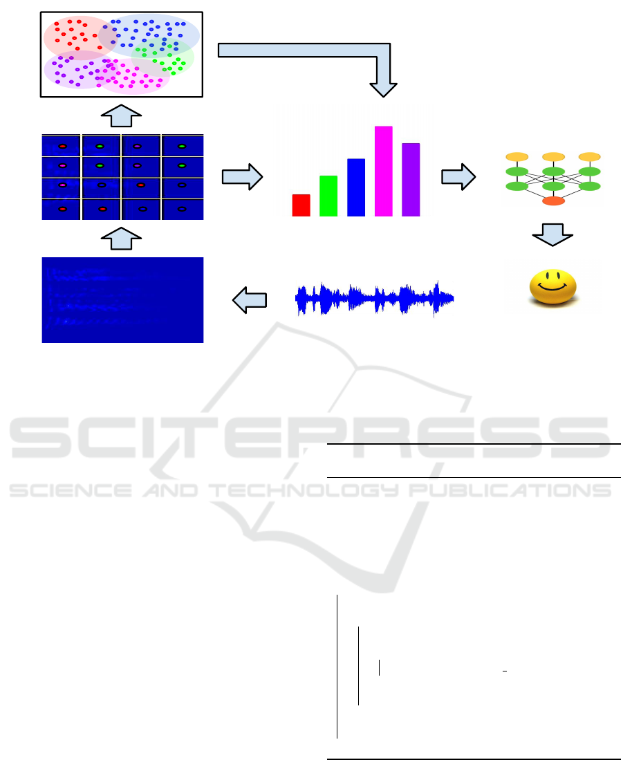
Figure 2: A visual overview of the proposed signal representation for our emotion recognition scheme. A spectrogram
is produced from the audio signal and a grid of keypoints characterized by ORB descriptors is constructed. Clustering
of keypoint descriptors is performed, leading to a vocabulary of visual words corresponding to the obtained clusters. A
soft histogram is obtained by summing the soft candidacy scores of keypoint descriptors to each cluster. The resulting
representation can be fed into a classifier to recognise a speaker’s affective state. (Figure best viewed in color).
of the visual words appearing in each column of the
spectrogram. In more detail, after each descriptor in
the spectrogram is matched to a visual word, each col-
umn of descriptors (including keypoints at all scales)
is converted to a soft histogram. The spectrogram is
then represented as the sequence of soft-histograms
appearing in its columns.
This sequential representation consisting of soft
histograms, encodes more information than the sim-
ple BoVW representation, which is insensitive to ran-
dom permutations of the columns of the spectrogram.
Such permutations of the columns lead to a spectro-
gram corresponding to an entirely different audio sig-
nal than the original, yet, both will have the same
BoVW representation. In other words, information
about the temporal structure of the audio signal is pre-
served by our sequential representation. As such, our
procedure may potentially boost the performance of
classifiers.
Our methodology for this section is described in
more detail in Procedure 2 and in Figure 3. The
spectrogram descriptors and visual vocabulary are ob-
tained by following the same steps as in Procedure 1.
Recurrent neural network architectures have
shown great success in processing sequential data and
are thus a natural candidate model for for processing
Procedure 2: Pseudocode for sequential soft-histogram
representation of spectrograms.
Input: Data of subsampled audio signals D,
parameter set λ;
Result: Sequential soft histogram representation
of elements in D;
ˆ
D,words ← Procedure 1(D,λ);
seqH ← {};
for each set of descriptors d in
ˆ
D do
seq ← [ ];
for each column of descriptors c in d do
histo ←
~
0;
for each descriptor d in c do
histo ← histo + soft score(d,words);
end
seq.append(histo)
end
seqH ← seqH ∪ {seq};
end
spectrograms in our sequential representation.
Among other architectures, in our methodology
and experiments we propose a Long Short-Term
Memory (LSTM) network for emotion classification
(Hochreiter and Schmidhuber, 1997). These networks
Sentiment Analysis from Sound Spectrograms via Soft BoVW and Temporal Structure Modelling
365

contain memory cells which are defined by the fol-
lowing equations, as presented by Sak et al.:
i
t
= σ(W
ix
x
t
+W
im
m
t−1
+W
ic
c
t−1
+ b
t
)
f
t
= σ(W
f x
x
t
+W
f m
m
t−1
+W
f c
c
t−1
+ b
f
)
c
t
= f
t
c
t−1
+ i
t
g (W
cx
x
t
+W
cm
m
t−1
+ b
c
) (5)
o
t
= σ(W
ox
x
t
+W
om
m
t−1
+W
oc
c
t
+ b
o
)
m
t
= o
t
h (c
t
)
y
t
= φ(W
ym
m
t
+ b
y
)
which, when applied iteratively for a given input se-
quence (x
1
,...,x
T
), produce a corresponding output
sequence (y
1
,...,y
T
) (Sak et al., 2014). This archi-
tecture is capable of recognising long-term dependen-
cies between items in the sequence, while also being
superior to alternative recurrent architectures in this
aspect.
4 EXPERIMENTS
In this section we describe the experimental proce-
dure we followed to provide evidence for the effec-
tiveness of our proposed methods in the sentiment
recognition problem. Our experiments are split in
two rounds. In the first round, our aim is to show
that using soft histograms in the usual bag of words
model (Spyrou et al., 2019), provides better results
with fewer visual words. In the second round our aim
is to combine the ideas from section 3.4 to create a
classifier that outperforms the simple BoVW models,
even using soft histograms.
For all our experiments, visual words were ob-
tained from the spectrograms using the mini-batch k-
means algorithm (Sculley, 2010). In particular, the
entire corpus was used for each dataset to extract the
words, i.e., the validation and test set too. In prac-
tice this can always be done; once we have a dataset
on which we want to recognise emotion, we can con-
struct a new pool of words which utilizes information
(through an unsupervised algorithm) from the unla-
beled set to improve prediction performance.
4.1 Datasets
The datasets utilized in our experiments consist of
the following popular emotion recognition datasets:
EMO-DB (Burkhardt et al., 2005), SAVEE (Jackson
and ul haq, 2011) and EMOVO (Costantini et al.,
2014). The considered emotions in our experiments
were Happiness, Sadness, Anger, Fear and Neutral
which were common to all considered datasets. For
each dataset and sample corresponding to these emo-
tions, a spectrogram was constructed from the corre-
sponding audio file, and a 50-by-50 grid of keypoints
was used at three different scales for a total of 7500
descriptors per recording. The spectrograms which
were extracted from the audio files corresponding to
each dataset can be seen in Figure 1.
4.2 Experimental Procedure
4.2.1 Feature Representation Comparison
For the first round of experiments, we evaluated
our soft histogram representation using three popular
classifiers: SVM (with an RBF kernel), Random For-
est and k-nearest neighbors with Euclidean distance
as a proximity measure. Each was trained in the emo-
tion recognition task on different representations of
the dataset; soft and simple histograms resulting from
different pools of visual words. We also evaluated the
regular BoVW representation, in order to have a base-
line for comparison with our method.
We performed a 90% − 10% train-test split on
each dataset. For each representation, the values
of hyperparameters for each of the considered clas-
sifiers, were also selected through grid search and
cross-validation over the training set. In particular,
we used 5 folds for cross validation. For each combi-
nation of hyperparameters, the one attaining the high-
est average accuracy among all folds was chosen as
the best. After obtaining the hyperparameters, the re-
sulting classifier was trained on the entire training set,
and evaluated on the test set. In addition, three differ-
ent numbers of visual words were used and the entire
evaluation was repeated for each. These were 250,
500 and 1000.
4.2.2 Classification Benchmarking
In this section we describe our methodology for the
second round of experiments. We built a recur-
rent neural network model using Long-Short Term
Memory (LSTM) units (Hochreiter and Schmidhu-
ber, 1997) to classify spectrograms represented as
sequences of soft histograms (see section 3.4). A
simple evaluation procedure was repeated for each
dataset and each choice of the number of visual words
used. A bidirectional LSTM network with a single
layer was used as a feature extractor and and a multi-
label logistic regression model was used on top for
classification. For each trial, an 80% − 10% − 10%
train-validation-test split was made and the model was
trained on the training set using an early-stopping
callback for regularization, which monitored the ac-
curacy on the validation set. In particular, the accu-
racy on the validation set was monitored with a pa-
tience of 15 epochs.
ICPRAM 2020 - 9th International Conference on Pattern Recognition Applications and Methods
366

Table 1: Results for the first round of experiments, where the histogram and soft-histogram representations are compared.
Dataset W.C. Method SVM KNN Random
Forest
EMO-DB
250
SMH 47.22 50.00 38.89
BoVW 44.44 33.33 38.89
500
SMH 52.78 41.67 52.78
BoVW 52.78 38.89 50.00
1000
SMH 55.56 47.50 55.00
BoVW 52.50 47.50 52.50
SAVEE
250
SMH 31.25 31.25 25.00
BoVW 28.13 31.25 25.00
500
SMH 52.78 48.89 61.11
BoVW 52.78 44.44 61.11
1000
SMH 58.33 52.78 58.33
BoVW 55.56 36.11 55.56
EMOVO
250
SMH 35.00 32.50 35.00
BoVW 30.00 27.50 32.50
500
SMH 32.50 42.50 35.00
BoVW 27.50 27.50 32.50
1000
SMH 32.50 40.00 50.00
BoVW 27.50 17.50 45.00
Table 2: Results for classification benchmarking experiment. Accuracies are given in percentages. W.C. represents word
count and B represents the benchmark obtained from the previous round of experiments.
Dataset W.C.
Accuracy
B
Mean Max Min
EMO-DB
250 59.76 60.98 58.54 50.00
500 62.93 63.17 60.54 52.78
1000 56.48 57.34 56.10 55.56
SAVEE
250 37.77 44.44 30.55 31.25
500 65.08 69.16 62.22 61.11
1000 68.77 70.55 66.39 58.33
EMOVO
250 40.91 42.86 38.90 35.00
500 50.98 57.14 47.62 42.50
1000 50.12 53.64 46.53 50.00
The resulting model was evaluated on the test set
and 10 trials were made for each word count-dataset
setup. The mean, maximum and minimum achieved
accuracies are listed as percentages and contrasted
with the benchmarks obtained in the first round of ex-
periments.
4.3 Results
The observed results on both experiments are in line
with our expectations. For the first round, the soft
histogram representation is indeed found to aid clas-
sification for all tested classifiers relative to the simple
histogram representation. The results are summarized
in Table 1. In the second round of experiments, we
observe the added value of the sequential represen-
tation of spectrograms, through the much better ob-
tained classifiers relative to the BoVW model from
experiment 1. The results are summarized in Table 2.
We observe that although there is a significant in-
crease in performance when going from a vocabu-
lary size of 250 to 500 for both methods, the perfor-
mance change when increasing the vocabulary size
from 500 to 1000 is not significant and may even
lead to decreased performance. This is possibly be-
cause the signal-to-noise ratio is decreased for too
large visual vocabularies and this provides additional
evidence that using soft histogram representations is
beneficial, since it leads to increased performance for
fewer words.
5 CONCLUSIONS
There is an increasing interest in emotion recognition
from audio signals, as sound recordings can be col-
Sentiment Analysis from Sound Spectrograms via Soft BoVW and Temporal Structure Modelling
367
…………………
...
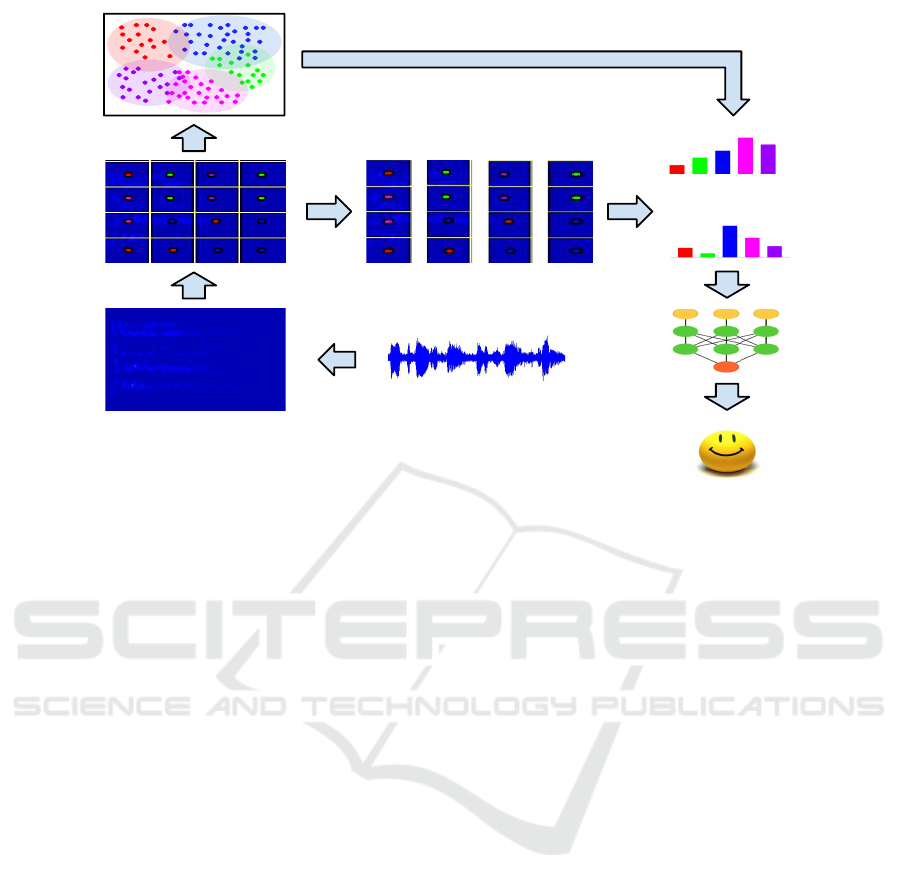
Figure 3: A visual overview of the proposed sequential representation for our emotion recognition scheme. Similar steps to
procedure 1 are taken to produce a visual vocabulary. Then each column of the spectrogram, corresponding to a temporal
“position” of the sliding window used in the DTSTFT transformation of the audio signal is converted to soft histogram in the
obvious manner. The sequence of soft histograms produced for a single audio signal is the passed to an LSTM classifier to
recognise the speaker’s sentiment. (Figure best viewed in color).
lected without causing as much discomfort to the un-
derlying subjects as other methods (e.g., video, body
sensors e.t.c.). For this reason, we have explored
new methods for analyzing audio signals of vocalized
speech for the purpose of recognizing the affective
state exhibited by the speaker, which build on spec-
trogram analysis methods found in the literature.
We conclude that the proposed approaches to sen-
timent recognition from sound spectrograms offer a
significant improvement over previous work. In par-
ticular, by combining the soft histogram representa-
tion of visual words along with temporal structure
modelling, we are able to obtain much better classi-
fiers in terms of accuracy. Another upside is that we
replaced the use of SIFT/SURF (which previous work
utilized) with ORB, which is a free alternative, with-
out loss in model quality.
Overall, the explored approach to emotion recog-
nition offers good performance on data collected
through a non-invasive method and can be found use-
ful in many HCI applications including assisted liv-
ing and personalizing content. Moreover, because our
method relies on low-level features (spectrograms) it
leads to language independent models and we have
empirically verified its good performance on two dif-
ferent languages (English and German) for the same
sentiment analysis tasks.
ACKNOWLEDGEMENTS
This research has been co-financed by the European
Union and Greek national funds through the Oper-
ational Program Competitiveness, Entrepreneurship
and Innovation, under the call RESEARCH – CRE-
ATE – INNOVATE (project code: 1EDK-02070).
REFERENCES
Anagnostopoulos, C.-N., Iliou, T., and Giannoukos, I.
(2015). Features and classifiers for emotion recog-
nition from speech: a survey from 2000 to 2011. Ar-
tificial Intelligence Review, 43(2):155–177.
Bay, H., Tuytelaars, T., and Van Gool, L. (2006). Surf:
Speeded up robust features. In European conference
on computer vision, pages 404–417. Springer.
Binali, H., Wu, C., and Potdar, V. (2010). Computational
approaches for emotion detection in text. In 4th IEEE
International Conference on Digital Ecosystems and
Technologies, pages 172–177. IEEE.
Burkhardt, F., Paeschke, A., Rolfes, M., Sendlmeier, W. F.,
and Weiss, B. (2005). A database of german emotional
speech. In Ninth European Conference on Speech
Communication and Technology.
Busso, C., Bulut, M., Lee, C.-C., Kazemzadeh, A., Mower,
E., Kim, S., Chang, J. N., Lee, S., and Narayanan,
ICPRAM 2020 - 9th International Conference on Pattern Recognition Applications and Methods
368

S. S. (2008). Iemocap: Interactive emotional dyadic
motion capture database. Language resources and
evaluation, 42(4):335.
Costantini, G., Iadarola, I., Paoloni, and Todisco, M.
(2014). Emovo corpus: an italian emotional speech
database.
Cowie, R., Douglas-Cowie, E., Tsapatsoulis, N., Votsis,
G., Kollias, S., Fellenz, W., and Taylor, J. G. (2001).
Emotion recognition in human-computer interaction.
IEEE Signal processing magazine, 18(1):32–80.
El Ayadi, M., Kamel, M. S., and Karray, F. (2011). Sur-
vey on speech emotion recognition: Features, classi-
fication schemes, and databases. Pattern Recognition,
44(3):572–587.
Giannakopoulos, T. and Pikrakis, A. (2014). Introduction
to audio analysis: a MATLAB
R
approach. Academic
Press.
Hochreiter, S. and Schmidhuber, J. (1997). Long short-term
memory. Neural computation, 9(8):1735–1780.
Jackson, P. and ul haq, S. (2011). Surrey audio-visual ex-
pressed emotion (savee) database.
Jin, Q., Li, C., Chen, S., and Wu, H. (2015). Speech emo-
tion recognition with acoustic and lexical features.
In 2015 IEEE international conference on acoustics,
speech and signal processing (ICASSP), pages 4749–
4753. IEEE.
Lim, W., Jang, D., and Lee, T. (2016). Speech emotion
recognition using convolutional and recurrent neural
networks. In 2016 Asia-Pacific Signal and Informa-
tion Processing Association Annual Summit and Con-
ference (APSIPA), pages 1–4. IEEE.
Lowe, D. G. (2004). Distinctive image features from scale-
invariant keypoints. International journal of computer
vision, 60(2):91–110.
Mao, Q., Dong, M., Huang, Z., and Zhan, Y. (2014). Learn-
ing salient features for speech emotion recognition us-
ing convolutional neural networks. IEEE transactions
on multimedia, 16(8):2203–2213.
Mehrabian, A. (1995). Framework for a comprehensive de-
scription and measurement of emotional states. Ge-
netic, social, and general psychology monographs.
Nogueiras, A., Moreno, A., Bonafonte, A., and Mari
˜
no,
J. B. (2001). Speech emotion recognition using hid-
den markov models. In Seventh European Conference
on Speech Communication and Technology.
Plutchik, R. (1980). A general psychoevolutionary theory of
emotion. In Theories of emotion, pages 3–33. Elsevier.
Poria, S., Chaturvedi, I., Cambria, E., and Hussain, A.
(2016). Convolutional mkl based multimodal emo-
tion recognition and sentiment analysis. In 2016
IEEE 16th international conference on data mining
(ICDM), pages 439–448. IEEE.
Rozgi
´
c, V., Ananthakrishnan, S., Saleem, S., Kumar, R.,
Vembu, A. N., and Prasad, R. (2012). Emotion recog-
nition using acoustic and lexical features. In Thir-
teenth Annual Conference of the International Speech
Communication Association.
Rublee, E., Rabaud, V., Konolige, K., and Bradski, G. R.
(2011). Orb: An efficient alternative to sift or surf. In
ICCV, volume 11, page 2. Citeseer.
Sak, H., Senior, A., and Beaufays, F. (2014). Long short-
term memory recurrent neural network architectures
for large scale acoustic modeling. In Fifteenth annual
conference of the international speech communication
association.
Sculley, D. (2010). Web-scale k-means clustering. In
Proceedings of the 19th international conference on
World wide web, pages 1177–1178. ACM.
Spyrou, E., Nikopoulou, R., Vernikos, I., and Mylonas, P.
(2019). Emotion recognition from speech using the
bag-of-visual words on audio segment spectrograms.
Technologies, 7(1):20.
Theodoridis, S. and Koutroumbas, K. D. (1999). Pattern
recognition. IEEE Trans. Neural Networks, 19:376.
Trentin, E., Scherer, S., and Schwenker, F. (2015). Emo-
tion recognition from speech signals via a probabilis-
tic echo-state network. Pattern Recognition Letters,
66:4–12.
Wang, Y. and Guan, L. (2008). Recognizing human emo-
tional state from audiovisual signals. IEEE transac-
tions on multimedia, 10(5):936–946.
W
¨
ollmer, M., Metallinou, A., Eyben, F., Schuller, B., and
Narayanan, S. (2010). Context-sensitive multimodal
emotion recognition from speech and facial expres-
sion using bidirectional lstm modeling. In Proc. IN-
TERSPEECH 2010, Makuhari, Japan, pages 2362–
2365.
Zeng, E., Mare, S., and Roesner, F. (2017). End user se-
curity and privacy concerns with smart homes. In
Thirteenth Symposium on Usable Privacy and Secu-
rity ({SOUPS} 2017), pages 65–80.
Sentiment Analysis from Sound Spectrograms via Soft BoVW and Temporal Structure Modelling
369
