
Securing Industrial Production from Sophisticated Cyberattacks
Andrew Sundstrom
a
, Damas Limoge
b
, Vadim Pinskiy
c
and Matthew Putman
d
Nanotronics Imaging, Brooklyn, NY, U.S.A.
Keywords:
Cyberattack, Malicious Attack, Man-in-the-Middle, Stuxnet, Statistical Process Control, Machine Learning,
Artificial Intelligence, Innovation Error, Deep Reinforcement Learning.
Abstract:
Sophisticated industrial cyberattacks focus on machine level operating systems to introduce process variations
that are undetected by conventional process control, but over time, are detrimental to the system. We pro-
pose a novel approach to industrial security, by treating suspect malicious activity as a process variation and
correcting for it by actively tuning the operating parameters of the system. As threats to industrial systems
increase in number and sophistication, conventional security methods need to be overlaid with advances in
process control to reinforce the system as a whole.
1 INTRODUCTION
The past 30 years of cyberattacks have witnessed a
startling degree of proliferation, adaptation, speci-
ficity, and sophistication
1
(see Figure 1). Industrial
and military security is the study of walls, physi-
cal and digital, which limit malicious insertion or re-
moval of information. For high-security factories and
military installations, this means creating systems that
are removed from the global computer network and
often removed from internal networks. Minuteman
ICBM silos, for example, are entirely isolated sys-
tems whose launch protocols are seldom updated and
whose launch directives are delivered over the Strate-
gic Automated Command and Control System
2
—
both protocol and directive systems have relied
3,4
, un-
til recently
5,6
, on data stored on 8-inch floppy disks,
employing an effective combination of network iso-
lation, obsolete IBM Series/1 computing hardware,
and low-capacity digital media that is too small for
a sophisticated modern cyberattack with a large code
footprint. Factory systems (e.g. PLC (Laughton and
a
https://orcid.org/0000-0002-3378-4513
b
https://orcid.org/0000-0002-4963-0500
c
https://orcid.org/0000-0002-5899-1172
d
https://orcid.org/0000-0002-1045-1441
1
https://bit.ly/36BjOkt
2
https://bit.ly/3041w91
3
https://bit.ly/2tDxtZE
4
https://wapo.st/2FvgNGp
5
https://bit.ly/2QXUJJR
6
https://nyti.ms/2QAojWP
Warne, 2003) and SCADA (Boyer, 2009)) operate on
static code that has been validated and is assumed to
be immutable, if not by foreign manipulation. In this
study, we focus on an industrial setting to describe our
approach.
Although computer methods can be used for vali-
dation and security verification prior to deployment,
the actual evidence of malicious code installation
comes from in-field testing of the entire production
line. If malicious code is installed, conventional the-
ory says its effects should manifest themselves in the
overall yield of the production line. This method of
statistical detection is typically successful in catch-
ing direct cyberattacks on single nodes, but it fails
against more sophisticated, systemic cyberattacks.
The best known example of the new breed of so-
phisticated cyberattacks
7,8
is Stuxnet
9
(Karnouskos,
2011), which surfaced in 2010
10
. The effects on the
centrifuges infected by Stuxnet were not statistically
significant with respect to expected baseline behavior,
and so each piece of hardware passed nominal Statis-
tical Process Control (SPC) standards. Even if one
machine—a single node—starts to behave atypically,
7
https://bit.ly/39P5gQ9
8
https://bit.ly/2s6iaIt
9
https://bit.ly/36zw056
10
For a detailed account, refer to the Repository of Indus-
trial Security Incidents (RISI) database, which records “in-
cidents of a cyber security nature that have (or could have)
affected process control, industrial automation or Super-
visory Control and Data Acquisition (SCADA) systems.”
https://www.risidata.com/
Sundstrom, A., Limoge, D., Pinskiy, V. and Putman, M.
Securing Industrial Production from Sophisticated Cyberattacks.
DOI: 10.5220/0009148206630670
In Proceedings of the 6th International Conference on Information Systems Security and Privacy (ICISSP 2020), pages 663-670
ISBN: 978-989-758-399-5; ISSN: 2184-4356
Copyright
c
2022 by SCITEPRESS – Science and Technology Publications, Lda. All rights reserved
663

the effects would manifest in the outputs of that node,
measured against historical averages, and the machine
would be immediately taken offline, before the entire
process can be affected or before other machines can
be similarly infected.
In sophisticated modern cyberattacks, however,
SPC is ill-suited to detect subtle changes in the op-
eration of many system elements, which individu-
ally have small changes, and are thus undetected,
but when integrated over time, have major and often
catastrophic effects on the entire system. To counter
this vulnerability, we propose several methods for de-
tection or correction, based on learning distributions
of the system and identifying anomalous behavior. In
the corrective case, an agent continuously runs the
feedback and feed-forward controls of the system, si-
multaneously correcting for nominal process varia-
tions (e.g. those that occur as a result of process or
raw material quality fluctuations) and preventing ma-
licious cyberattacks.
Figure 1: The growth in the number of distinct cyberattacks
in the past 30 years, as depicted by Kaspersky Labs.
2 STATISTICAL PROCESS
CONTROL
Statistical Process Control (SPC), as popularized by
William Edwards Deming in post-war Japan (Dem-
ing and Renmei, 1951), (Deming, 1986), (Denton,
1991), (Delsanter, 1992), calls for process standards
to be established for each step in the manufacturing
process and monitored throughout the production life
cycle. The goal is to continuously improve the pro-
cess through the life cycle.
It is assumed that as long as each node is oper-
ating within specification, the final product will also
be within specification. The specifications are set
based on subject matter expertise and historical per-
formance. The dependability and impact of one node
onto the next or subsequent nodes is not directly ad-
justed in SPC, but rather, each sub-process is exam-
ined as an independent entity. This leads to wider
margins for the operating condition of each node, pre-
venting the system from ever operating in the absolute
highest efficiency or stability.
From a security perspective, this margin can be
targeted by sophisticated process cyberattacks. If a
single node or several nodes in a system start to op-
erate at the upper bounds (or lower bounds) of their
specification, individual alarms will not be triggered,
but the overall process quality will be affected. This
especially holds for man-in-the-middle cyberattacks,
where reported sensor signals, for example, are faked
by the malicious code. The life cycle of the node will
also be affected, requiring increased downtime for re-
pair. Several layers of downstream nodes will also be
affected and over time, the continual drift of the sys-
tem will tend toward non-compliance. By that point,
the correction needed to recover the system would be
massive and cost-prohibitive.
3 A MATHEMATICAL MODEL
OF PROCESS CONTROL
DISRUPTION
A factory can be defined using to a wide variety of
topological schemes, including feedback and feed-
forward organization. Here we give a simple model
of a factory, offering just enough complexity to facili-
tate a rigorous presentation of the approaches outlined
below, which can operate on system topologies of ar-
bitrary complexity.
Accordingly, we define a factory, F, as a strictly
linear sequence of n processing nodes, labeled
1,...,n, connected in a forward-linked chain.
F :→ 1 →2 →···→i → ···→ n
The processing done by each node i has two at-
tribute distributions, an expected distribution, Q
i
, and
an observed distribution, P
i
. Q
i
is characterized by µ
Q
i
and σ
Q
i
. If Q
i
= N(µ
Q
i
,σ
2
Q
i
), then Q
i
is completely
characterized. P
i
is characterized by µ
P
i
and σ
P
i
. If
P
i
= N(µ
P
i
,σ
2
P
i
), then P
i
is completely characterized.
We define the damage caused by node i to be the
Kullback–Leibler divergence (Kullback and Leibler,
1951), (Kullback, 1959) of P
i
with respect to Q
i
:
d
i
= D
KL
(P
i
||Q
i
) =
∑
x∈χ
P
i
(x)log
P
i
(x)
Q
i
(x)
. (1)
ICISSP 2020 - 6th International Conference on Information Systems Security and Privacy
664
For this simple, illustrative model, we assume
damage is cumulative, more specifically additive,
across F, and so
d
F
=
n
∑
i=1
d
i
. (2)
Consider the Statistical Process Control (SPC)
protocol, which uses µ
i
and σ
i
to determine if pro-
cessing at node i is in or out of control on the basis of
whether x ∈P
i
falls within µ
Q
i
±3σ
Q
i
.
Now consider two adversarial cases for node i,
where Q
i
= N(µ
Q
i
,σ
2
Q
i
) and P
i
= N(µ
P
i
,σ
2
P
i
):
• Case 1 (max-burn): µ
P
i
= µ
Q
i
+ 3σ
Q
i
− ε
i
and
σ
P
i
=
ε
i
5
• Case 2 (min-burn): µ
P
i
= µ
Q
i
−3σ
Q
i
+ε
i
and σ
P
i
=
ε
i
5
By setting σ
P
i
=
ε
i
5
, we ensure 99.99943% of the
observed events stay in control.
This gives a definition of SPC satisfaction:
SPCSAT = 1(
1
n
n
∑
i=1
1({x :x ∈ P
i
|
µ
P
i
±5σ
P
i
and
x 6∈Q
i
|
µ
Q
i
±3σ
Q
i
} = ∅) > τ
s
),
(3)
for some ratio τ
s
∈(0, 1], typically 1, meaning the pro-
cessing of all nodes 1,...,n is in control.
By definition, Cases 1 and 2 satisfy SPC; their P
i
burn at, but are safely contained within, the upper and
lower bounds of the Q
i
, respectively.
Despite satisfying SPC, Cases 1 and 2 do accu-
mulate measurable damage. This is the essence of
how a cyberattack like Stuxnet works; it causes pro-
cessing nodes to operate within established statistical
tolerances, while accumulating damage to the manu-
factured products.
Consider Case 1. The probability density func-
tions for Q
i
and P
i
are given by
q
i
(x) =
1
q
2πσ
2
Q
i
e
−
(x−µ
Q
i
)
2
2σ
2
Q
i
(4)
and
p
i
(x) =
1
q
2π(
ε
i
5
)
2
e
−
(x−(µ
Q
i
+3σ
Q
i
−ε
i
))
2
2(
ε
i
5
)
2
, (5)
respectively.
Since most of the probability mass of P
i
is near
x = µ
Q
i
+ 3σ
Q
i
−ε
i
and is otherwise close to 0 (see
Figure 2), we find
q
i
(x) ≈
1
q
2πσ
2
Q
i
e
(3σ
Q
i
−ε
i
)
2
2σ
2
Q
i
(6)
and
p
i
(x) ≈
1
q
2π(
ε
i
5
)
2
. (7)
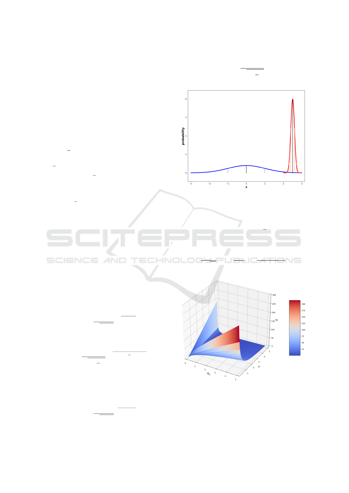
Figure 2: Example expected distribution Q
i
(blue) and ex-
ample observed distribution P
i
(red) for a given node i in
Case 1: P
i
is designed to occupy the rightmost extreme
subrange of Q
i
, where the probability mass of P
i
for x ∈
µ
P
i
±5σ
P
i
is entirely contained within x ∈ [µ
Q
i
+ 3σ
Q
i
−
2ε
i
,µ
Q
i
+ 3σ
Q
i
]. Shown here: {µ
Q
i
= 0, σ
Q
i
= 1}, {ε
i
=
0.5,µ
P
i
= µ
Q
i
+ 3σ
Q
i
−ε
i
= 2.5, σ
P
i
=
ε
i
5
= 0.1}.
Substituting these into the definition of d
i
, we derive
d
i
=
5
ε
i
√
2π
log
5σ
Q
i
ε
i
+
(ε
i
−3σ
Q
i
)
2
2σ
Q
i
. (8)
Figure 3: Damage, d
i
, as a function of expected standard de-
viation, σ
Q
i
and proximity to SPC tolerance, ε
i
, for a given
node i in Cases 1 and 2, as given by (8).
We depict (8) in Figure 3. Here we see that as ex-
pected variance, σ
Q
i
, shrinks to 0 while proximity to
Securing Industrial Production from Sophisticated Cyberattacks
665

SPC tolerance, ε
i
, grows, then damage, d
i
increases
exponentially. Similarly, as ε
i
shrinks to 0 while σ
Q
i
grows, then d
i
increases exponentially. These two
maxima represent two intuitively undesirable situa-
tions, neither of which are detected by SPC: {σ
Q
i
→
0,ε
i
→ ∞} =⇒ the stringency of Q
i
outstrips the
proximity of P
i
to the extrema of Q
i
; and {σ
Q
i
→
∞,ε
i
→ 0} =⇒ P
i
occupies an ever-narrowing sub-
range of Q
i
.
Consider Case 2. The only difference from Case
1 is the probability density function for P
i
, given by
p
i
(x) =
1
q
2π(
ε
i
5
)
2
e
−
(x−(µ
Q
i
−3σ
Q
i
+ε
i
))
2
2(
ε
i
5
)
2
. (9)
Since most of the probability mass of P
i
is near
x = µ
Q
i
−3σ
Q
i
+ε
i
and is otherwise close to 0, we find
p
i
(x) is identical to Case 1, so the remaining deriva-
tion follows identically, as one expects from the sym-
metric normal distribution.
Hence, in Cases 1 and 2, we have an expression
that defines a measurable damage for each node i in F
despite their having satisfied SPC. Sufficiently large
cumulative damage implies process control disrup-
tion:
d
F
> τ
d
. (10)
4 FORMULATING THE DAMAGE
RECOVERY PROBLEM
SPC is a static, non-interventional approach to pro-
cess control, where well-defined statistical properties
are passively observed to pass or fail at each node,
and only after the last node’s processing is a decision
made as to whether to keep or discard the manufac-
tured product.
By contrast, we consider a dynamic, interven-
tional approach to process control, where each node
subsequent to the node causing detected damage is
woven into an optimization problem—the damage re-
covery problem–and actively controlled to instantiate
a solution to it. This is done near real-time and while
each cycle is ongoing, rather than at the end of a given
cycle.
If a control system detects node k has caused
damage (i.e., has produced a damaged or distorted
distribution), then intuitively, we want to employ a
control strategy that samples from P
k
, and generates
all subsequent resulting distributions flowing from it,
P
k+1
,...,P
n
, such that the remaining cumulative dam-
age, d
k+1
+ ···+ d
n
, is minimized. Accordingly, we
formulate the damage recovery problem as
argmin
{P
k+1
,...,P
n
}
(
n
∑
i=k+1
D
KL
(P
i
||Q
i
)
)
. (11)
5 PROPOSED SOLUTION
ARCHITECTURES
In the interest of minimizing the damage, D
KL
, as
defined in (11), one might consider simply applying
more stringent controls to each node of the process,
effectively minimizing the σ
Q
i
, or attempt to idealize
the situation by assuming zero (or nearly zero) ob-
servable variance in practice, effectively minimizing
the σ
P
i
. More stringent controls translate into expo-
nential increases in expense in the number of nodes,
n, and observing ideally low levels of variance may
very well be impossible over long time spans for any
realistic manufacturing process.
As a counter to the trivial solution above, several
advanced methods for detection or correction are con-
sidered. One naturally follows the other, though a
correction method may include only implicit detec-
tion. Three potential solutions to the correction of
damage are outlined below, though their efficacy will
be explored later. The first uses adaptive methods
to control a system with an unknown disturbance, in
the simplest case, a constant disturbance. To gener-
alize the distribution description from (1), a single-
input, single-output system is established in state-
space form as
˙
~x
i
= A
i
~x
i
+ B
i
u
ε,i
(t)
y
i
(t) = C
>
i
~x
i
,
(12)
for ~x
i
defined as arbitrary states of the system, y de-
fined as the output of the system, and A, B and C
are system matrices defining the ordinary differential
equation of the underlying dynamics. The input of
this system, u
ε
, is a noisy input signal defined by
u
ε,i
= u
i
(t) + ε
t
, (13)
where ε
t
is additive noise contributed by ε
t
∼
N (µ
ε,i
,R
i
) Additionally, the observed output, y
ν
, is
a function of the system output in (12) as
y
ν,i
= y
i
(t) + ν
t
(14)
for a similarly noisy signal measurement, with ν
t
∼
N (µ
ν,i
,σ
2
ν,i
). This notation is reconciled with that of
Sections 3 – 4 by establishing that y
ν,i
∼Q
i
for a given
node, i, of a process. In an unaffected system, the
mean of the noise contributions are zero, such that
µ
ε,i
= µ
ν,i
= 0. In a malicious cyberattack, however,
the deviation manifests as non-zero mean input noise.
ICISSP 2020 - 6th International Conference on Information Systems Security and Privacy
666

5.1 Innovation Error Distribution via
Kalman Filter State Estimation
A common approach to estimating states within a sys-
tem similar to (12) is a Kalman Filter (Kalman, 1960)
(KF), which can be extended to nonlinear systems as
well. The formulation of the KF is generally reliant
on zero mean noise, but in the case of a malicious
cyberattack, the offset of the input instruction would
manifest as a non-zero mean additive noise. There-
fore, a KF can be constructed for the presumed linear
time-invariant system described in (12). The filter is
constructed using measurements of output, y
ν,i
(t) for
a node of a process, and the canonical, untouched in-
put instructions u
i
(t). If the process is correctly cali-
brated, the input/output sensor measurements should
have zero mean noise, but in the case of a malicious
cyberattack there would be a non-zero bias, as de-
picted in Figure 2. The filter (Thrun et al., 2005) is
constructed as
¯
~x
i,k
= A
i
ˆ
~x
i,k−1
+ B
i
u
i,k
¯
Σ
i,k
= A
i
Σ
i,k−1
A
>
i
+ R
i
K
i,k
=
¯
Σ
i,k
C
i
(C
>
i
¯
Σ
i,k
C
i
+ σ
2
ν,i
)
−1
ˆ
~x
i,k
=
¯
~x
i,k
+ K
i,k
(y
ν,i,k
−C
>
i
¯
~x
i,k
)
Σ
i,k
= (I −K
i,k
C
>
i
)
¯
Σ
i,k
(15)
for the k
th
sample of a process node, i, where ¯· is
the measurement update notation, Σ
i,k
is the covari-
ance of the state prediction, R
i
is the covariance of
the input noise, ε
t
, and K
i,k
are the Kalman gains.
With a large enough sample, the innovation distribu-
tion, ˜y
i,k
= y
ν,i,k
−C
>
i
¯
~x
i,k
should be ˜y
i,k
∼ N (µ
˜y,i,k
=
0,C
>
i
Σ
i,k|k−1
C
i
). However, with a malicious cyber-
attack, µ
˜y,i,k
6= 0, but this can occur naturally with
minimal samples. Once a sample threshold is met,
k > k
min
, an alarm can be established for ˜y
i,k
> γ
i
,
where γ
i
can be tuned for a process node. If the in-
novation error is non-zero and above the threshold γ
i
,
a malicious cyberattack might be occurring. Figure 4
shows a schematic of the filter described in (15). It
should be noted that a twin controller must be main-
tained and isolated from the primary PLC controllers.
This is used as an unbiased reference for the kalman
filter. The limitations of this method are requiring a
known system, of the form A, B, and C. Addition-
ally, the duplicated controller represent an additional
challenge for maintaining software links. To alleviate
these issues, agnostic inferential methods can be used
as abstract representations of the system node.
y
s
A(s)
Σ
−
C(s) G(s)
y
ν,i,k
H(s)
Σ
C(s) KF
˜y
i,k
Figure 4: A block diagram of the systems described in (12),
incorporating the Kalman filter of (15) for innovation error
distribution. The controller, C(s), the plant, G(s), and the
measurement, H(s), represent the basic constituents of the
nodal control, while the Kalman filter, KF, produced an in-
novation error. The attack is represented by the block A(s).
5.2 Inferential Methods for Detection
and Correction
Artificial Intelligence (AI) (Russell and Norvig,
2010) in the form of Deep Learning (DL) (Goodfel-
low et al., 2016) has revolutionized image processing
(Krizhevsky et al., 2012), machine translation (John-
son et al., 2017), and many other forms of classifica-
tion (Goodfellow et al., 2014). Specifically, the abil-
ity to form complex and non-obvious associations be-
tween image pixels and labels, has allowed for higher
accuracy of detection than conventional computer vi-
sion (Krizhevsky et al., 2012). These methods are also
not constrained by the same matching conditions of
classical filter methods, such as approach suggested
in Section 5.1. This enables more availability for sys-
tems that have undetermined or hard to model dynam-
ics.
5.2.1 Autoencoding for Unsupervised Anomaly
Detection
Significant attention has been paid to autoencoders
trained to detect anomalies (An and Cho, 2015),
(Sakurada and Yairi, 2014), (Zhou and Paffenroth,
2017), which, when paired with a Long Short-
Term Memory (LSTM) (Hochreiter and Schmidhu-
ber, 1997) block in both the encoder and decoder,
has been shown to be applicable to anomaly detec-
tion. In (Malhotra et al., 2016), an autoencoder was
constructed with these LSTM blocks which maintain
a state memory of the sequence. For a sequence of
measured outputs, ~y
ν,i
, an unsupervised autoencoder
training can be instantiated to map the entropy of out-
put observations on to a parameter set, θ
AE
, such that
ˆ
~y
ν,i
= f (~y
ν,i
,θ
AE
). (16)
The error of this autoencoder is defined as
˜
~y
ν,i
=~y
ν,i
−
ˆ
~y
ν,i
, (17)
Securing Industrial Production from Sophisticated Cyberattacks
667

and for a normal operation,
˜
~y
ν,i
∼N (µ
˜y,i
,Σ
˜y,i
), where
µ
˜y
and Σ
˜y,i
are fit to the distribution using maximum
likelihood. Subsequently, an anomaly score, a
i
, for a
sequence can be defined as
a
i
= A
˜
~y
ν,i
,µ
˜y,i
,Σ
˜y,i
= (
˜
~y
ν,i
−µ
˜y,i
)
>
Σ
−1
˜y,i
(
˜
~y
ν,i
−µ
˜y,i
).
(18)
Similarly to the Kalman Filter formulation in Section
5.1, when the anomaly score, a
i
> γ
i
, an anomaly is
detected and an alarm is sounded. Figure 5 shows a
block diagram of the autoencoder system. The limi-
y
s
A(s)
Σ
−
C(s) G(s)
y
ν,i,k
H(s)
Σ
AE
a
i
A
Figure 5: A block diagram of the systems described in (16)–
(18), incorporating the autoencoder for anomaly detection.
The controller, C(s), the plant, G(s), and the measurement,
H(s), represent the basic constituents of the nodal control,
while the autoencoder, AE, detects errors, wherein a suffi-
cient anomaly score triggers alarm A. The attack is repre-
sented by the block A(s).
tations of the autoencoder approach are a reliance on
node-specific training of trajectory prediction models,
ignoring the complete factory output. It is possible
that while one node is operating appropriately, a pre-
vious node has already created damage, and the out-
put of the node in question will already be affected.
To correct for this, a more complete system would
consider states of each nodal output as an entire tra-
jectory, and adjust the set-point input of each subse-
quent node accordingly. Such an approach could be
accomplished through online optimization methods,
such as reinforcement learning.
5.2.2 Deep Reinforcement Learning
In Sections 5.1 and 5.2.1, malicious cyberattack de-
tection was discussed, but no implicit correction was
established. However, the definition of damage, d
i
,
given in (1) suggests a natural structure to formu-
late a delayed reward function for a reinforcement
learning agent seeking to construct a set of distri-
butions, P
k+1
,...,P
n
, to solve the damage recovery
problem given in (11), through its actions,
~
α
( j)
i
, for i =
k + 1,. . . , n, over some set of iterations, j = 1,. . . , m:
R(
~
α
( j)
) =
n
∑
i=k+1
r
i
(
~
α
( j)
i
), (19)
for
r
i
(
~
α
( j)
i
) = P
i
(
~
α
( j)
i
)log
P
i
(
~
α
( j)
i
)
Q
i
(
~
α
( j)
i
)
!
(20)
In (Lillicrap et al., 2015a), an agent is trained in an
actor-critic modality, such that one network produces
an action, α
i,k
, given a state, ~x
i,k
for the k
th
sample of
the i
th
node of a process, and another network makes
a prediction of Q-value, Q
π
i,k
(~x
i,k
,α
i,k
|θ
Q,i
), learned
over parameters θ
Q,i
, where π
i
(~x
i,k
,θ
π,i
) is a learned
policy over parameters θ
π,i
. The reward is calculated
using a Bellman formulation such that
Q
i
(~x
i,k
,α
i,k
) = r
i,k
+ γ
i
Q
i
(~x
i,k+1
,π
i
(~x
i,k+1
)|θ
π,i
).
(21)
Most reinforcement learning agents use an update
law corresponding to maximizing the expected return.
However, given the formulation in (11), our update
law will be
−∇
θ
π,i
J =
−E
α
i,k
∼ρ
[∇
α
i
Q
i
(~x
i,k
,α
i,k
|θ
Q,i
)∇
θ
π
π
i
(~x
i,k
|θ
π,i
)].
(22)
This update law will minimize the Q-value, thereby
minimizing damage, and will manifest in actions
aimed at returning the distribution to its canonical
shape. One formulation of action could be
u
i,k
= α
i,k
u
∗
i,k
, (23)
where u
i,k
is the input of (12), α
i,k
is an instruction
modifier, and u
∗
i,k
is the instruction read for a partic-
ular sample, k, of node i. If this instruction is cor-
rupted, and that corruption manifests in the states, the
policy, π
i,k
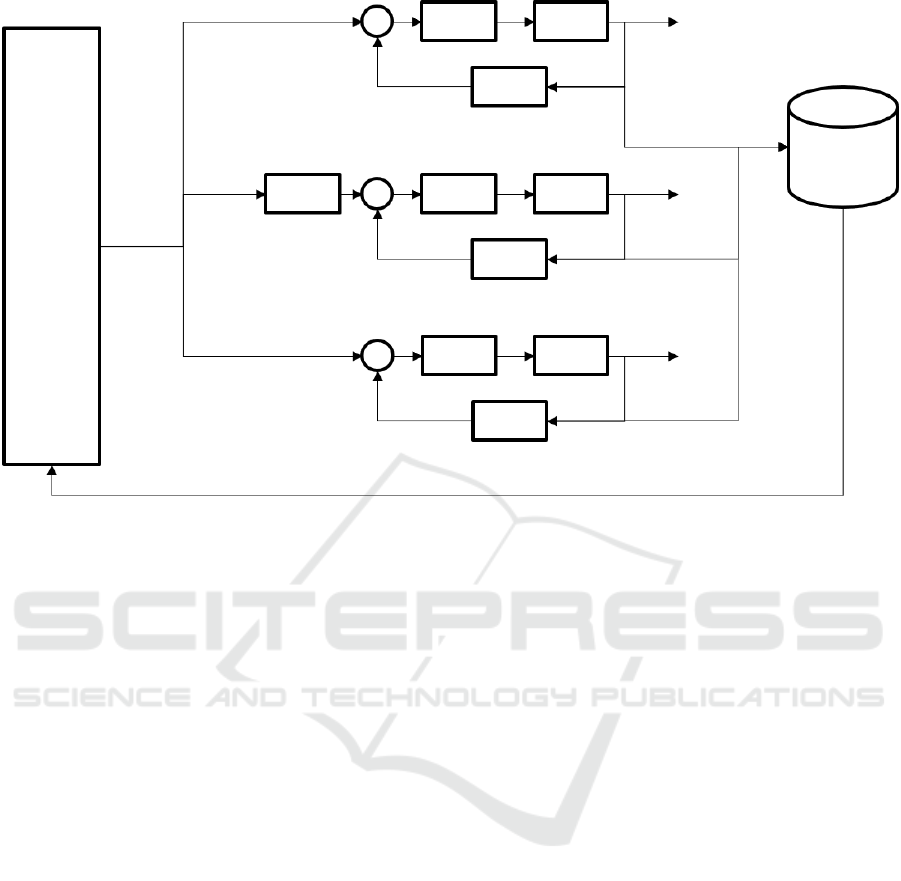
, will act to correct it. Figure 6 shows a
scheme to operate the agent within a factory setting,
acting as an outer-loop for the control set-point. An
alternative version would directly vary the gain of the
control effort from the C
i
(s) controllers, subverting
the set-point input.
Reinforcement learning has proven effective in
complex environments (Sutton and Barto, 2018), (Lil-
licrap et al., 2015b), (Schulman et al., 2017), (Fuji-
moto et al., 2018), but requires significant samples to
converge. It is recommended that an agent is tuned
on simulation data first, then subsequently refined on
observed data, before it is deployed in a live system.
Moreover, this approach offers a new way to ad-
dress system security by bundling process-based ma-
licious cyberattacks into nominal process variations
and offers direct control and correction for those vari-
ations. The approaches is not simply a method of de-
tection or passive prevention; rather, a cyberattack is
assumed to manifest as a routine (e.g. probable) sys-
tem variation, such as a machine tuning out of norm or
a raw material stock moving out of tight specification.
ICISSP 2020 - 6th International Conference on Information Systems Security and Privacy
668
Σ
Σ
Σ
A(s)
y
s,0,k
y
s,i,k
y
s,N,k
−
−
−
C
0
(s)
C
i
(s)
C
N
(s)
G
0
(s)
G
i
(s)
G
N
(s)
H
0
(s)
H
i
(s)
H
N
(s)
y
ν,0,k
y
ν,i,k
y
ν,N,k
Y
π(S
k
)
S
k
Figure 6: A block diagram of a potential scheme for reinforcement learning based manufacturing control of multiple nodes,
i = 0,. . . , N. For each node i, the controller, C
i
(s), the plant, G
i
(s), and the measurement, H
i
(s), represent the basic constituents
of the nodal control. Together, the nodes are embedded in a policy-learning feedback loop governed by the state of the system
at time k, S
k
, sampled from data store Y , and the policy taking the current state as input, π(S
k
). The attack is represented for
a single node, i, by the block A(s).
One would not know that the system was infected,
but as long as the agent is making active controls, the
final product would be unchanged and the effect of
the cyberattack nullified. This also creates latency for
nominal IT process to take place and detect intrusion.
By focusing on active process control, rather than re-
active models, this approach takes advantage of time
series data throughout the manufacturing process and
not just a single data point for each finished good.
6 CONCLUSION
Physical and digital detachment, which has largely
shielded industrial equipment from immediately
catastrophic malicious cyberattacks, is no longer suf-
ficient for cyber-defense. In order to enable dis-
tributed manufacturing measurement, analysis and
feedback, process nodes must be networked, present-
ing a cyberattack vector for nefarious actors. Even
with sophisticated firewalls and real-time alarms to
detect corrupted process trajectories, an opportunity
persists for minimally invasive alterations to process
instructions to operate within acceptable statistical
tolerances while damaging the final product irrepara-
bly. The answer is not to deprecate the functional-
ity of modern factories in the interest of safeguard-
ing their output, nor is it to pour immense capital into
process nodes to ensure their operation fits within an
impenetrable distribution of operation.
More sophisticated cyberattacks are able to pen-
etrate standalone equipment, inserting process varia-
tions and commands, causing subtle, non-trivial er-
rors that are difficult to detect through conventional
process control methods. These cyberattacks can
be planned months or years before the actual effect
on the instrumentation—possibly within the supply
chain of the equipment—making detection and pre-
vention difficult to impossible. The effects they intro-
duce are time and process-state integrative over long
scales and across multiple nodes, making detection
and correction difficult. We present several alterna-
tive approaches for a generalized manufacturing set-
ting that offer not only complete standalone operation,
but also active correction for all types of process vari-
ation. A sophisticated cyberattack on a specific node
or a change in the raw material is corrected by ac-
tively changing the processing conditions of subse-
quent nodes. This agent is continually operational,
regardless of the cyberattack, and prevents malicious
attempts to alter the steady-state processing from hav-
ing a noticeable effect on the final quality of the sys-
tem. This approach increases quality and yield of the
Securing Industrial Production from Sophisticated Cyberattacks
669

system by actively correcting for all types of nomi-
nal variations, while offering increased resistance to
possible cyberattacks on the process equipment.
REFERENCES
An, J. and Cho, S. (2015). Variational autoencoder based
anomaly detection using reconstruction probability.
Special Lecture on IE, 2(1).
Boyer, S. A. (2009). SCADA: Supervisory Control And
Data Acquisition. International Society of Automa-
tion, USA, 4 edition. ISBN 1936007096.
Delsanter, J. (1992). Six sigma. Managing Service Quality,
2(4).
Deming, W. E. (1986). Out of Crisis. MIT Center for Ad-
vanced Engineering Study, Cambridge, MA, USA.
Deming, W. E. and Renmei, N. K. G. (1951). Elementary
Principles of the Statistical Control of Quality; a Se-
ries of Lectures. Tokyo, Nippon Kagaku Gijutsu Rem-
mei, Tokyo, Japan.
Denton, D. (1991). Lessons on competitiveness: Motorola’s
approach. Production and Inventory Management
Journal, 32(3).
Fujimoto, S., van Hoof, H., and Meger, D. (2018). Ad-
dressing function approximation error in actor-critic
methods. arXiv preprint arXiv:1802.09477.
Goodfellow, I., Bengio, Y., and Courville, A. (2016). Deep
Learning. MIT Press, Cambridge, MA, USA. ISBN
0262035618. http://www.deeplearningbook.org.
Goodfellow, I. J., Pouget-Abadie, J., Mirza, M., Xu, B.,
Warde-Farley, D., Ozair, S., Courville, A., and Ben-
gio, Y. (2014). Generative adversarial nets. In
Proceedings of the 27th International Conference on
Neural Information Processing Systems - Volume 2,
NIPS’14, pages 2672–2680, Cambridge, MA, USA.
MIT Press.
Hochreiter, S. and Schmidhuber, J. (1997). Long short-term
memory. Neural Computation, 9(8):1735—-1780.
Johnson, M., Schuster, M., Le, Q. V., Krikun, M., Wu, Y.,
Chen, Z., Thorat, N., Vi
´
egas, F., Wattenberg, M., Cor-
rado, G., Hughes, M., and Dean, J. (2017). Google’s
multilingual neural machine translation system: En-
abling zero-shot translation. Transactions of the Asso-
ciation for Computational Linguistics, 5:339–351.
Kalman, R. E. (1960). A new approach to linear filtering
and prediction problems. Journal of basic Engineer-
ing, 82(1):35–45.
Karnouskos, S. (2011). Stuxnet worm impact on indus-
trial cyber-physical system security. In 37th Annual
Conference of the IEEE Industrial Electronics Society
(IECON 2011), Melbourne, Australia. http://papers.
duckdns.org/files/2011 IECON stuxnet.pdf.
Krizhevsky, A., Sutskever, I., and Hinton, G. E. (2012).
Imagenet classification with deep convolutional neu-
ral networks. In Pereira, F., Burges, C. J. C., Bot-
tou, L., and Weinberger, K. Q., editors, Advances
in Neural Information Processing Systems 25, pages
1097–1105. Curran Associates, Inc. https://bit.ly/
39PWOAb.
Kullback, S. (1959). Information Theory and Statistics.
John Wiley & Sons.
Kullback, S. and Leibler, R. (1951). On information
and sufficiency. Annals of Mathematical Statistics,
22(1):79–86.
Laughton, M. and Warne, D., editors (2003). Electrical En-
gineer’s Reference Book, chapter 16. Newnes, 16 edi-
tion. ISBN 0750646373.
Lillicrap, T. P., Hunt, J. J., Pritzel, A., Heess, N., Erez, T.,
Tassa, Y., Silver, D., and Wierstra, D. (2015a). Contin-
uous control with deep reinforcement learning. arXiv
preprint arXiv:1509.02971.
Lillicrap, T. P., Hunt, J. J., Pritzel, A., Heess, N., Erez,
T., Tassa, Y., Silver, D., and Wierstra, D. (2015b).
Continuous control with deep reinforcement learning.
arXiv preprint arXiv:1509.02971.
Malhotra, P., Ramakrishnan, A., Anand, G., Vig, L., Agar-
wal, P., and Shroff, G. (2016). LSTM-based encoder-
decoder for multi-sensor anomaly detection. arXiv
preprint arXiv:1607.00148.
Russell, S. and Norvig, P. (2010). Artificial Intelligence: A
Modern Approach. Prentice Hall, Upper Saddle River,
NJ, USA, 3 edition. ISBN 0136042597. http://aima.
cs.berkeley.edu/.
Sakurada, M. and Yairi, T. (2014). Anomaly detection
using autoencoders with nonlinear dimensionality re-
duction. In Proceedings of the MLSDA 2014 2nd
Workshop on Machine Learning for Sensory Data
Analysis, page 4. ACM.
Schulman, J., Wolski, F., Dhariwal, P., Radford, A., and
Klimov, O. (2017). Proximal policy optimization al-
gorithms. arXiv preprint arXiv:1707.06347.
Sutton, R. S. and Barto, A. G. (2018). Reinforcement
Learning: An Introduction. MIT Press, Cambridge,
MA, USA, 2 edition. ISBN 0262039249. http://
incompleteideas.net/book/the-book-2nd.html.
Thrun, S., Burgard, W., and Fox, D. (2005). Probabilistic
robotics. MIT press.
Zhou, C. and Paffenroth, R. C. (2017). Anomaly detec-
tion with robust deep autoencoders. In Proceedings of
the 23rd ACM SIGKDD International Conference on
Knowledge Discovery and Data Mining, pages 665–
674. ACM.
ICISSP 2020 - 6th International Conference on Information Systems Security and Privacy
670
