Dynamic Mode Decomposition via Dictionary Learning for Foreground

Modeling in Videos

Israr Ul Haq

, Keisuke Fujii

1,2

and Yoshinobu Kawahara

1,3

Center for Advanced Intelligence Project, RIKEN, Japan

Graduate School of Informatics, Nagoya University, Japan

Institute of Mathematics for Industry, Kyushu University, Fukuoka, Japan

Keywords:

Dynamic Mode Decomposition, Nonlinear Dynamical System, Dictionary Learning, Object Extraction,

Background Modeling, Foreground Modeling.

Abstract:

Accurate extraction of foregrounds in videos is one of the challenging problems in computer vision. In this

study, we propose dynamic mode decomposition via dictionary learning (dl-DMD), which is applied to extract

moving objects by separating the sequence of video frames into foreground and background information with

a dictionary learned using block patches on the video frames. Dynamic mode decomposition (DMD) decom-

poses spatiotemporal data into spatial modes, each of whose temporal behavior is characterized by a single

frequency and growth/decay rate and is applicable to split a video into foregrounds and the background when

applying it to a video. And, in dl-DMD, DMD is applied on coefﬁcient matrices estimated over a learned

dictionary, which enables accurate estimation of dynamical information in videos. Due to this scheme, dl-

DMD can analyze the dynamics of respective regions in a video based on estimated amplitudes and temporal

evolution over patches. The results on synthetic data exhibit that dl-DMD outperforms the standard DMD and

compressed DMD (cDMD) based methods. Also, the results of an empirical performance evaluation in the

case of foreground extraction from videos using publicly available dataset demonstrates the effectiveness of

the proposed dl-DMD algorithm and achieves a performance that is comparable to that of the state-of-the-art

techniques in foreground extraction tasks.

1 INTRODUCTION

One of the fundamental computer vision objectives is

to extract accurate dynamic information from video

sequences. The basic application can be the sepa-

ration of foreground and background information in

videos. This is still considered to be a challenging

task in practice because the true background is of-

ten difﬁcult to estimate. To address this issue, vari-

ous methods have been proposed over the last decade.

For detailed overview of some of the traditional and

state-of-the-art methods, we recommend (Bouwmans

et al., 2017; Sobral and Vacavant, 2014). One of

the most extensively used frameworks to separate a

video into foreground and background information is

decomposing the video frames into a low-rank ma-

trix (background) and a sparse matrix (foreground)

by principal component analysis (PCA) (Oliver et al.,

1999). Variants of this method, such as robust prin-

cipal component analysis (RPCA), are further dis-

cussed in (Cand

es et al., 2011). The decomposition

of a matrix into low-rank and sparse matrices can

be alternatively solved by dynamic mode decomposi-

tion (DMD), which accurately separates a matrix into

the stationary background and foreground motions

by differentiating between the near-zero frequency

modes and the remaining non-zero frequency modes

(Kutz and Fu, 2015). However, there are some limita-

tions in the standard DMD method that often causes

inaccurate extraction of dynamics from the video. In

standard DMD method, image sequences ordered in

time as column vectors are considered as input, such

arrangement of image sequences is unable to extract

complex dynamics in videos. Also a modiﬁed version

of standard DMD; compressed DMD (cDMD) have

been proposed in (Erichson et al., 2016). The com-

pressed DMD achieves almost the same results as the

standard DMD method but at low computation cost.

In this study, we advocate the use of DMD via

dictionary learning (dl-DMD) for accurate extraction

of dynamics in videos. For this purpose, a dictio-

nary is learned using random patches of input image

476

Haq, I., Fujii, K. and Kawahara, Y.

Dynamic Mode Decomposition via Dictionary Learning for Foreground Modeling in Videos.

DOI: 10.5220/0009144604760483

In Proceedings of the 15th International Joint Conference on Computer Vision, Imaging and Computer Graphics Theory and Applications (VISIGRAPP 2020) - Volume 5: VISAPP, pages

476-483

ISBN: 978-989-758-402-2; ISSN: 2184-4321

sequences for better approximation of the input sig-

nals. Then coefﬁcient matrices are obtained over this

learned dictionary those contain the better represen-

tation of underlying dynamics in videos which results

in a sharp extraction of foreground structures from the

background than standard DMD and cDMD.

The remainder of this study can be organized as

follows. First, we provide an overview of the dynamic

mode decomposition in Section 2. Then in Section 3,

we describe a problem formulation and procedure to

perform dl-DMD. Experiments are presented in Sec-

tion 4 along with performance evaluations. Finally,

Section 5 summarizes and concludes the study.

2 DYNAMIC MODE

DECOMPOSITION

DMD spatiotemporally decomposes the sequential

data via data-driven realization of the spectral decom-

position of the Koopman operator (Koopman, 1931).

Spectral analysis of the Koopman operator lifts the

analysis of nonlinear dynamical systems to those of

linear systems in function spaces. Further, we brieﬂy

review the underlying theory.

Consider a (possibly nonlinear) dynamical sys-

tem:

t+1

= f

f (x

), x

x ∈ M ,

where f

M → M , M is the state space, and t is the

time index. In this system, the Koopman operator K

for ∀x

x ∈ M can be deﬁned as follows:

K g(x

x) = g( f

f (x

x)),

where g

M → C (∈ F ) denotes an observable in

function space F . By deﬁnition, K is a linear op-

erator in F . Assume that there exists a subspace of

F invariant to K , which can be denoted by G ⊂ F .

Additionally, assume that G is ﬁnite-dimensional and

that a set of observables {g

,... ,g

} that span over G

are observed to exist. If g

g = [g

,. .. ,g

]

M → C

the one-step evolution of g

g for ∀x

x ∈ M can be ex-

pressed as follows:

g(x

x) = g

g( f

f (x

x)),

where the ﬁnite dimensional K

K is the restriction of

K to G. An eigenfunction of K

K can be expressed as

M → C

, and the corresponding eigenvalue can

be expressed as λ ∈ C, i.e., K

Kϕ

ϕ(x

x) = λϕ

ϕ(x

x). If all

eigenvalues are distinct, any value of g

g can be ex-

pressed as follows:

g(x

x) =

∑

i=1

ϕ(x

x)ξ

with some coefﬁcients ξ

. Thus, we obtain

Algorithm 1 : Dynamic Mode Decomposition (Schmid,

2010).

Require: Y

and Y

deﬁned in Eq. (1)

Ensure: Dynamic modes Φ

Φ and eigenvalues ∆

∆

1: U

← compact SVD of Y

A ← U

∗

−1

W ,∆

∆

∆ ← eigenvectors and eigenvalues of

4: Φ

Φ ← Y

−1

5: return: Φ

Φ,∆

∆

∆;

Algorithm 2: Compressed Dynamic Mode Decomposition.

Require: Video frames Y

1: R

R = rand(p

,m)  Generate sensing matrix

2: Y

= R

R*Y

, Y

R*Y

 Compress input matrix

3: U

U,S

S,V

V = svd(Y

)  SVD

4: A

A = U

U * Y

V *S

−1

 Least squares ﬁt

5: W

W ,∆

∆

∆ = eig(A

A)  Eigenvalue decomposition

6: Φ

= Y

∗V

V ∗ S

−1

∗W

W  Compute DMD modes

7: b

b = lstsq(Φ

Φ,Y

)  Compute amplitudes by least

square method

g(x

) =

∑

i=1

, c

= ϕ

)ξ

where g

g is decomposed into modes {c

}, and the mod-

ulus and argument of λ

express the decay rate and

frequency of c

, respectively. Differing from classical

modal decomposition of linear systems, this decom-

position can be applied to nonlinear systems. DMD

computes such decomposition using the numerical

data. Assume the following data matrices of sizes

n×T

= [g

g(x

),. ..,g

g(x

T −1

)],

= [g

g(x

),. ..,g

g(x

)].

(1)

Then, the most popular variant of the DMD al-

gorithm is described in Algorithm 1. In compressed

DMD (cDMD) method, data matrices are ﬁrst com-

pressed by a random sensing matrix and then modes

are reconstructed using the original data matrix. The

algorithm is further summarized in Algorithm 2.

3 PROPOSED METHOD

We propose dl-DMD by extending DMD to employ

the dictionary atoms that have been learned using ran-

dom patches in video frames. The dictionary learning

step allows the reconstruction of input video frames

using a small subset of dictionary atoms. Then, DMD

is performed over the coefﬁcient matrices those are

obtained over the dictionary atoms (explained in sub-

section. 3.2) which contain the better representation

of underlying dynamics of input video and expected

Dynamic Mode Decomposition via Dictionary Learning for Foreground Modeling in Videos

477

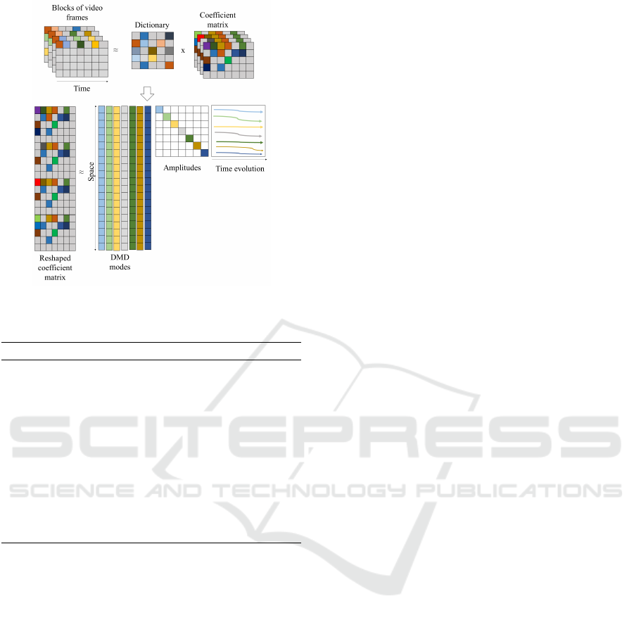
Figure 1: Illustration of dl-DMD for back-

ground/foreground separation in videos.

Algorithm 3: dl-DMD for foreground extraction in videos.

Require: Video frames V, patch size d, dictionary

atoms k.

1: Learn a dictionary D as in Eq. (2).

2: Calculate the coefﬁcient matrices B

and B

as in

Eqs. (3) and (4), respectively.

3: Perform DMD over coefﬁcient matrices B

and

(subsection 3.3).

4: Threshold zero-frequency modes based on the

eigenvalues obtained by Step 3.

5: Reconstruct foregrounds from the approximated

coefﬁcient matrix and dictionary as in Eq. (9).

to cause accurate foreground/background separation

based on the obtained eigenvalues and spatial modes

(explained in subsection 3.3). However, in stan-

dard DMD and cDMD methods, DMD is directly

applied over spatiotemporal matrices those are built

from input frames of a video due to which it be-

comes difﬁcult to extract dynamics and seperate fore-

ground/background information. The overall proce-

dure of dl-DMD is summarized in Algorithm 3, and

the proposed method is further illustrated in Figure 1.

The details of the main steps are described as follows:

3.1 Dictionary Learning

First, in case of a given video frames V ∈ R

×n

×T

each frame {v

,. .. ,v

} is converted to a set of

overlapping patches, and l patches from the entire set

are selected randomly to train a dictionary D ∈ R

d×k

where d is the size of a patch and k is the number of

atoms or elements in the dictionary. The dictionary

can be learned by optimizing the coefﬁcient matrix

Z ∈ R

k×l

and the dictionary in an iterative manner.

The dictionary and coefﬁcient matrix are estimated to

give a representation to approximate X ∈ R

d×l

, which

contains the randomly selected patches {x

}

j=1

in the

columns (Aharon et al., 2006). This can be performed

by solving the following minimization problem:

min

D,Z



kX − DZk



subject to ∀

,||z

≤ T

(2)

where the coefﬁcient matrix Z = {z

,. .. ,z

} contains

coefﬁcients that represent each patch and T

is the

maximum number of non-zero coefﬁcients that can

be used to represent each patch.

3.2 Coefﬁcient Matrix Estimation

The coefﬁcient matrices B

{

i,1

i,2

,. .. ,

i,(T −1)

}

i=1

and B

= {

i,1

i,2

,. .. ,

i,(T −1)

}

i=1

of sizes R

K×(T −1)

are learned

over the trained dictionary to approximate the patches

of image sequences Q

= {q

i,1

i,2

,. .. ,q

i,(T −1)

}

i=1

and Q

= {q

i,2

i,3

,. .. ,q

i,T

}

i=1

of sizes R

N×(T −1)

Here, {·}

i=1

is the vectorized column with the total

number of overlapping patches, P; further, N and

K represent the total number of rows in the aligned

frames and coefﬁcient matrices, respectively. The

patches along all the aligned frames are represented

as Q = {q

i, j

}

i=1

∈ R

N×T

for j = 1,...,T , and

those approximations can be obtained by solving the

following minimization problems:

i, j

= arg min

i, j

− Dβ

i, j

+ λ

kβ

i, j

(i = 1, 2,. .. ,P, j = 1,2, .. ., T − 1),

(3)

i, j

= arg min

i,( j−1)

i, j

− Dβ

i,( j−1)

+ λ

kβ

i,( j−1)

(i = 1, 2,. .. ,P, j = 2,. .. ,T ),

(4)

where λ

and λ

in Eqs. (3) and (4) denote the reg-

ularization parameters to control the sparsity in the

coefﬁcient matrices B

and B

, respectively.

3.3 Dynamic Mode Decomposition

The dynamic modes are computed by applying Algo-

rithm 1 to the coefﬁcient matrices B

and B

. A set

of dynamic modes Φ

= {φ

,. .. ,φ

} and the corre-

sponding eigenvalues ∆

∆

= {Λ

,. .. ,Λ

} are obtained,

those represent the spatial and frequency informa-

tion of the video. Here, r is the number of adopted

VISAPP 2020 - 15th International Conference on Computer Vision Theory and Applications

478

eigenvectors. These modes represent the slowly vary-

ing or rapidly moving objects at time points t ∈

{0,1, 2. .. ,T − 1} in the video frames with associated

continuous-time frequencies and can be expressed as

follows:

log(Λ

)

∆t

. (5)

Further, the approximated video frames for low- and

high-frequency modes at any time point can be recon-

structed as

B(t) ≈

∑

j=1

exp(ω

t)α

= Φ

Φexp(Ω

Ω

Ωt)α

α, (6)

where φ

is a column vector of the i-th dynamic mode

that contains the spatial structure information and α

is the initial amplitude of the corresponding DMD

mode. The vector of the initial amplitudes α

α can

be obtained by taking the initial video frame at time

t = 0, which reduces Eq. (6) to {

i,1

}

i=1

= Φ

Φα

α. Note

that the matrix of eigenvectors is not square; thus, the

initial amplitudes can be observed using the following

pseudoinverse process:

α = Φ

†

{

i,1

}

i=1

. (7)

3.4 Foreground/Background Separation

The key principle to separate the video frames into

foregrounds and the background is the thresholding

of low frequency modes based on the corresponding

eigenvalues. Generally, the portion that represents the

background is constant among the frames and satis-

ﬁes |ω

| ≈ 0, where p ∈ {1,2,..., r}. Typically, a

single mode represents the background, which is lo-

cated near the origin in the complex space, whereas

|ω

|,∀ j 6= p are the eigenvalues that represent the

foreground structures bounding away from the origin.

Therefore, the reconstructed video frames can be sep-

arated into the background and foreground structures

as follows:

B = φ

exp(ω

t)α

| {z }

Background

∑

j6=p

exp(ω

t)α

| {z }

Foreground

, (8)

where

B = {

i,1

i,2

,. .. ,

i,T

}

i=1

is the reconstructed

coefﬁcient matrix and t = {0,. .. ,T − 1} is the time

indices up to (T − 1) frames. Note that the initial

amplitude α

= φ

†

{

i,1

}

i=1

of the stationary back-

ground is constant for all the future time points,

whereas α

= φ

†

{

i,1

}

i=1

,∀ j 6= p are the initial am-

plitudes of varying foreground structures. However,

full ﬂattened approximated video sequences are re-

constructed with a learned dictionary (in subsection

3.1) by the following equation:

{

i, j

}

P,T

i=1, j=1

= D{

i, j

}

P,T

i=1, j=1

(9)

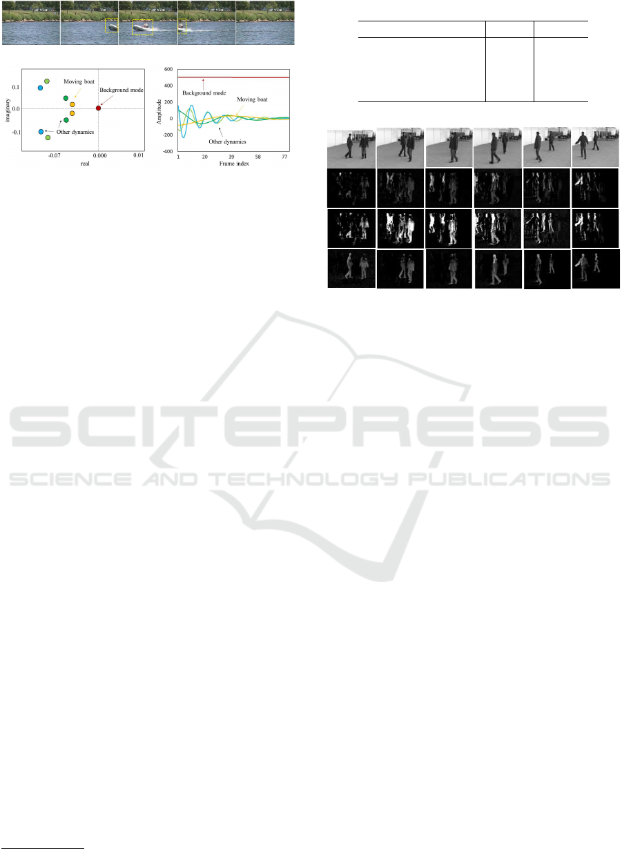
Foregrounds and background separation in a video

is illustrated in Figure 2, that depicts the continu-

ous time eigenvalues and temporal evolution of am-

plitudes (Erichson et al., 2016). Subplot (a) shows a

set of video frames of a moving boat

. It can be ob-

served that the boat is absent during the initial and

last frames, whereas the middle frame exhibits a full

moving boat. The representation of these frames into

modes that describe dynamics by applying dl-DMD

provides an interesting insight related to the moving

objects in the foreground, which can be achieved by

factorizing these frames into spatial modes, ampli-

tudes, and temporal evolutions. Subplot (b) exhibits

the different eigenvalues that are based on the infor-

mation present in the frames. The background is usu-

ally static in videos, which corresponds to the zero

eigenvalue that is located near the origin, whereas

the eigenvalues that are located away from the ori-

gin conﬁrm the presence of other dynamics. Further,

subplot(c) depicts the amplitude evolution and dic-

tates that the zero-frequency mode which is constant

over time, is the background, and that the remain-

ing modes, which correspond to different frequen-

cies, depict the foreground structures. Additionally,

we note that the amplitude that describes the moving

boat is negative in the initial frames and begins to in-

crease, eventually reaching its maximum at a frame

index of 40 when the boat is almost at the center of

the video, capturing majority of the foreground infor-

mation. The amplitude begins to decrease when the

boat moves away from the center. The remaining am-

plitudes with different frequencies describe the other

dynamics of the moving objects in the video.

4 EXPERIMENTAL RESULTS

We empirically investigated the performance of the

proposed dl-DMD using synthetic data (Section 4.1)

and a real video dataset, i.e., BMC (Section 4.2).

For the synthetic data, we compared our proposed dl-

DMD method with standard DMD and compressed

DMD because the comparative results of other algo-

rithms can be found in (Takeishi et al., 2017).

http://changedetection.net/

Dynamic Mode Decomposition via Dictionary Learning for Foreground Modeling in Videos

479

(a)

(b)

(c)

Figure 2: Splitting foreground and the background

(Changedetection.net (Goyette et al., 2012) video sequence

“boats”) . (a) ﬁve frames of a moving boat. (b) the near

zero eigenvalue corresponds to the background and rest to

other dynamics. (c) temporal evolutions of amplitudes.

4.1 Synthetic Data

We quantitatively evaluated the performance using

the synthetic data that were generated as follows.

First, a sequence of noisy images {s

∈ R

128×128

} was

generated using the following equation:

= e

+ e

+ N

, (10)

where p

, p

∈ R

128×128

and N

is the zero-mean

Gaussian noise with standard deviation σ = {0.3} for

t = 0,1, .. ., 15. The dynamic modes of the noise-

free image sequences are p

and p

, where e

= 0.99

and e2 = 0.9, are the corresponding eigenvalues, re-

spectively. The standard DMD, cDMD and dl-DMD

methods were applied on these noisy sequence of im-

ages. The comparison of these methods demonstrates

that the dl-DMD can approximate the underlying dy-

namics more accurately by estimating the true eigen-

values (e

) even in the presence of noise compared

to the standard DMD and cDMD. Table. 1 shows the

estimated eignevalues by standard, compressed and

dl-DMD method.

To demonstrate the effectiveness of the proposed

method visually, another experiment is performed

on a video of SBMnet

dataset, where people are

strolling in a terrace with no original background pro-

vided in the dataset. To visualize the foreground

structures extracted by the dl-DMD, standard and

cDMD methods we chose 200 consecutive frames

from the video and then applied all those three meth-

ods. Figure 3 (ﬁrst row) shows every 20th frame

of ﬁrst 100 frames of a video. Second row shows

the foregrounds extracted by standard DMD method.

Third and fourth rows show the foregrounds extracted

by the compressed DMD and the proposed method,

http://scenebackgroundmodeling.net/

Table 1: Estimated and the ground-truth eigenvalues.

Ground truth 0.99 0.9

Standard DMD 0.994 0.8319

Compressed DMD 0.994 0.8348

dl-DMD (proposed) 0.991 0.90

Figure 3: First-row: original video frames of moving peo-

ple; second-row: extracted foregrounds with standard DMD

method; Third-row: extracted foregrounds with compressed

DMD; Last-row: extracted foregrounds with dl-DMD (Pro-

posed).

respectively. It can be visualized that dl-DMD can

extract the foreground dynamics more accurately than

standard and cDMD methods. Note that, for this ex-

periment size of sensing matrix in cDMD was set to

= (n1 ∗ n2)/2 (see Algorithm 2), since too much

compression will result in loss of spatial information.

Parameters Selection: The parameters of dl-DMD

were tuned manually for best results and set to T

16, λ

,λ

= 10

−3

, dictionary size = 64 × 128, patch

size 8 ×8 with overlapping factor 1. A dictionary with

more number of dictionary atoms minimize the recon-

struction error after applying the DMD at the cost of

high computation time, whereas a dictionary with few

atoms holds less information that in result increases

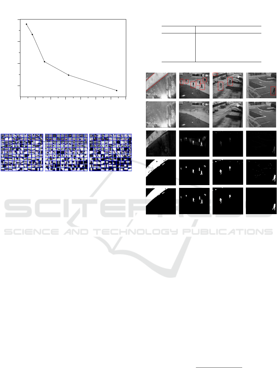
the reconstruction error. Figure. 4 shows the decrease

in reconstruction error by increasing the size of dictio-

nary atoms. Another important parameter is the patch

size, the relation between the patch size and the mean

reconstruction error (between the DMD reconstructed

output and input video) is shown in Table. 2. This

relation shows that for a ﬁxed number of dictionary

atoms, increasing the patch size results in increasing

the reconstruction error. Figure. 5 shows some of the

learned dictionaries on BMC dataset.

4.2 Real Video Dataset

We further measured the quantitative performance of

our proposed method on the publicly available BMC

dataset (Vacavant et al., 2012; Sobral and Vacavant,

VISAPP 2020 - 15th International Conference on Computer Vision Theory and Applications

480

Reconstruction Error

0.04

0.06

0.08

0.1

Number of Dictionary elements

0 20 40 60 80 100 120 140

Figure 4: Reconstruction error decreases with increasing

dictionary atoms.

Figure 5: Trained dictionaries on BMC dataset of ﬁrst three

videos; (001) Boring parking, (002) Big trucks and (003)

Wandering students.

2014). This dataset is a benchmark for background

modeling of various outdoor surveillance scenarios,

such as raining or snowing at different time inter-

vals, illumination changes or snowing at different

time intervals, illumination changes relative to out-

door lighting conditions, long duration of motionless

foreground objects, and dynamic backgrounds (e.g.,

moving clouds or trees).

Some of the foreground extraction results of BMC

videos (002), (003), (005) and (009) are shown in Fig-

ure 6 and evaluation results for all the nine videos

on this dataset are presented in Table. 3 (Erichson

et al., 2016). For pre-processing we cropped 200

consecutive frames of each video, and more than one

background is estimated for those videos where back-

ground changes with time as in videos (001), (005)

and (008).

These results indicate some of the strengths and lim-

itations of the proposed method. Note that the pro-

posed method is presented as a batch algorithm ap-

plied to a set of consecutive frames. Thus, any

changes that occur later in time are difﬁcult to de-

tect, such as the sleeping foreground in video (001),

when the cars are parked for a long period of time;

this reduces the F-measure value. Another factor

that reduces the F-measure value is the presence of

non-periodic backgrounds, such as snow and moving

clouds, which prominently appear in videos (005) and

(008), respectively. However, in case of videos with

Table 2: Relation b/w patch size and reconstruction error.

Patch size Reconstruction error

4 × 4 0.0326

8 × 8 0.0369

12 ×12 0.0373

16 × 16 0.0411

Figure 6: Foreground extraction corresponding to BMC

videos: 002, 003, 005 and 009. The top row shows a sin-

gle frame of each video. The second row shows the esti-

mated backgrounds. The third row shows the difference be-

tween the original frames and backgrounds reconstructed.

The fourth row shows the thresholded frames, and the ﬁfth

row shows the extracted foregrounds after applying mor-

phological operations (closing and dilation to ﬁll holes).

little variation in the background, high F-measure

values were obtained. The recall, precision, and F-

measure metrics were calculated to evaluate the real

videos.

Recall: It measures the ability to accurately detect the

foreground pixels which belong to the foreground.

Precision: It measures the number of accurately de-

tected foreground pixels which are actually correct.

F-measure: It is the harmonic mean of recall and pre-

cision that provides an average value when the values

are close, and calculated as

F = 2.

Precision × Recall

Precision + Recall

, (11)

dl-DMD achieves high F-measure values in videos

(003), (004) and (009) because the backgrounds of

these videos are almost static for the entire duration

and in video (002) background is static at different in-

Dynamic Mode Decomposition via Dictionary Learning for Foreground Modeling in Videos

481

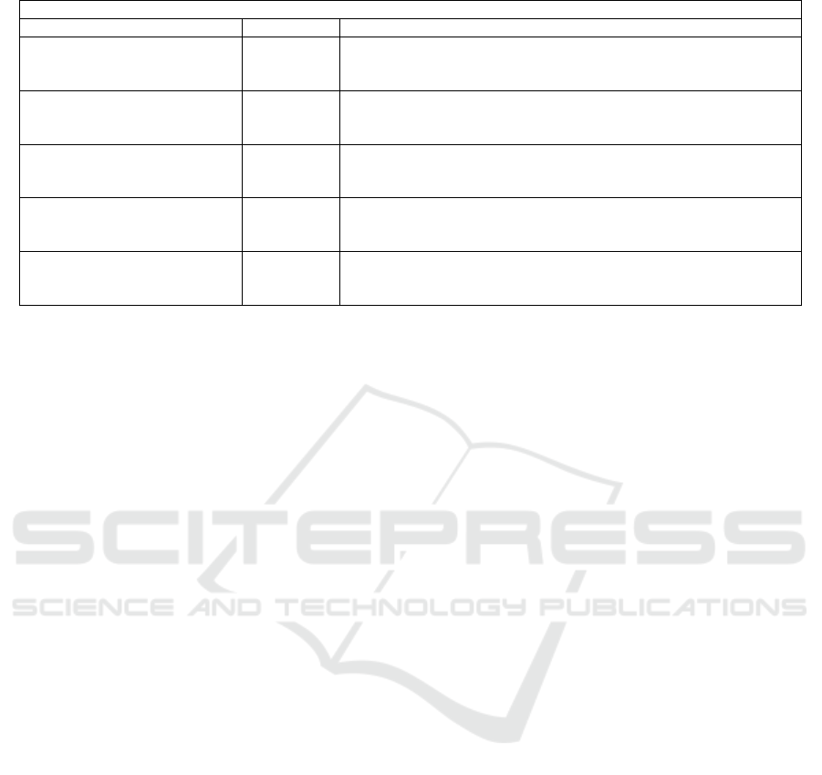
Table 3: Evaluation results (BMC dataset).

Measure BMC videos

001 002 003 004 005 006 007 008 009

Recall 0.800 0.689 0.840 0.872 0.861 0.823 0.658 0.589 0.690

RSL De La Torre Precision 0.732 0.808 0.804 0.585 0.598 0.713 0.636 0.526 0.625

(De La Torre and Black, 2003) F-Measure 0.765 0.744 0.821 0.700 0.706 0.764 0.647 0.556 0.656

Recall 0.693 0.535 0.784 0.721 0.643 0.656 0.449 0.621 0.701

LSADM Goldfarb Precision 0.511 0.724 0.802 0.729 0.475 0.655 0.693 0.633 0.809

et al.(Goldfarb et al., 2013) F-Measure 0.591 0.618 0.793 0.725 0.549 0.656 0.551 0.627 0.752

Recall 0.684 0.552 0.761 0.709 0.621 0.670 0.465 0.598 0.700

GoDec Zhou and Tao Precision 0.444 0.682 0.808 0.728 0.462 0.636 0.626 0.601 0.747

(Zhou and Tao, 2011) F-Measure 0.544 0.611 0.784 0.718 0.533 0.653 0.536 0.600 0.723

Recall 0.552 0.697 0.778 0.693 0.611 0.700 0.720 0.515 0.566

Erichson Precision 0.581 0.675 0.773 0.770 0.541 0.602 0.823 0.510 0.574

et al.(Erichson et al., 2016) F-Measure 0.566 0.686 0.776 0.730 0.574 0.647 0.768 0.512 0.570

Recall 0.584 0.732 0.806 0.882 0.493 0.608 0.565 0.456 0.713

dl-DMD (proposed) Precision 0.587 0.784 0.931 0.624 0.591 0.605 0.660 0.552 0.811

F-Measure 0.586 0.757 0.864 0.731 0.537 0.607 0.608 0.500 0.758

tervals of time. dl-DMD can extract small and large

moving foreground objects, such as a running rabbit

in video (004) and the big moving trucks with illumi-

nation changes in video (002), respectively; addition-

ally, the competitive F-measure values were obtained.

5 CONCLUSIONS

We proposed dl-DMD for accurate foreground extrac-

tion in videos. In dl-DMD, DMD is performed on

coefﬁcient matrices estimated over a dictionary that

is learned on the randomly selected patches from the

video frames. The experiments on synthetic data re-

veals that the use of dictionary with DMD can extract

complex dynamics in time series data more accurately

than standard DMD and cDMD methods. Also, ex-

periments on real video dataset demonstrates that our

proposed method can extract foreground and back-

ground information in videos with comparable per-

formance to other methods.

ACKNOWLEDGEMENTS

This work was supported by JSPS KAKENHI (Grant

Number JP18H03287) and JST CREST (Grant Num-

ber JPMJCR1913).

REFERENCES

Aharon, M., Elad, M., and Bruckstein, A. (2006). rmk-svd:

An algorithm for designing overcomplete dictionaries

for sparse representation. IEEE Transactions on Sig-

nal Processing, 54(11):4311–4322.

Bouwmans, T., Sobral, and Javed, S. (2017). Decompo-

sition into low-rank plus additive matrices for back-

ground/foreground separation. Computer Science Re-

view, 23:1–71.

Cand

es, E. J., Li, X., Ma, Y., and Wright, J. (2011). Robust

principal component analysis? Journal of the ACM

(JACM), 58(3):11.

De La Torre, F. and Black, M. J. (2003). A framework

for robust subspace learning. International Journal

of Computer Vision, 54(1-3):117–142.

Erichson, N. B., Brunton, S. L., and Kutz, J. N. (2016).

Compressed dynamic mode decomposition for back-

ground modeling. Journal of Real-Time Image Pro-

cessing, pages 1–14.

Goldfarb, D., Ma, S., and Scheinberg, K. (2013). Fast alter-

nating linearization methods for minimizing the sum

of two convex functions. Mathematical Programming,

141(1-2):349–382.

Goyette, N., Jodoin, P.-M., Porikli, F., Konrad, J., and Ish-

war, P. (2012). Changedetection. net: A new change

detection benchmark dataset. In CVPRW, 2012 IEEE

Computer Society Conference on, pages 1–8. IEEE.

Koopman, B. (1931). Hamiltonian systems and transfor-

mation in Hilbert space. Proceedings of the National

Academy of Sciences USA, 17(5):315–318.

Kutz, J. N. and Fu (2015). Multi-resolution dynamic mode

decomposition for foreground/background separation

and object tracking. In 2015 IEEE (ICCVW), pages

921–929. IEEE.

Oliver, N., Rosario, B., and Pentland, A. (1999). A bayesian

computer vision system for modeling human interac-

tions. In ICVS, pages 255–272. Springer.

Schmid, P. J. (2010). Dynamic mode decomposition of nu-

merical and experimental data. Journal of ﬂuid me-

chanics, 656:5–28.

Sobral, A. and Vacavant, A. (2014). A comprehensive re-

view of background subtraction algorithms evaluated

with synthetic and real videos. Computer Vision and

Image Understanding, 122:4–21.

Takeishi, N., Kawahara, Y., and Yairi, T. (2017). Sparse

non-negative dynamic mode decomposition. In 2017

VISAPP 2020 - 15th International Conference on Computer Vision Theory and Applications

482

IEEE Int. Conf. on Image Process. (ICIP’17), pages

2682–2686.

Vacavant, A., Chateau, T., Wilhelm, A., and Lequi

evre,

L. (2012). A benchmark dataset for outdoor fore-

ground/background extraction. In Asian Conference

on Computer Vision, pages 291–300. Springer.

Zhou, T. and Tao, D. (2011). Godec: Randomized low-

rank & sparse matrix decomposition in noisy case. In

ICML. Omnipress.

Dynamic Mode Decomposition via Dictionary Learning for Foreground Modeling in Videos

483