Simultaneous Object Detection and Semantic Segmentation

Niels Ole Salscheider

FZI Research Center for Information Technology, Karlsruhe, Germany

Keywords:

Autonomous Driving, Computer Vision, Deep Learning, Object Detection, Semantic Segmentation.

Abstract:

Both object detection in and semantic segmentation of camera images are important tasks for automated ve-

hicles. Object detection is necessary so that the planning and behavior modules can reason about other road

users. Semantic segmentation provides for example free space information and information about static and

dynamic parts of the environment. There has been a lot of research to solve both tasks using Convolutional

Neural Networks. These approaches give good results but are computationally demanding. In practice, a com-

promise has to be found between detection performance, detection quality and the number of tasks. Otherwise

it is not possible to meet the real-time requirements of automated vehicles. In this work, we propose a neural

network architecture to solve both tasks simultaneously. This architecture was designed to run with around

10 Hz on 1 MP images on current hardware. Our approach achieves a mean IoU of 61.2% for the semantic

segmentation task on the challenging Cityscapes benchmark. It also achieves an average precision of 69.3%

for cars and 67.7% for pedestrians on the moderate difﬁculty level of the KITTI benchmark.

1 INTRODUCTION

Automated vehicles need a detailed perception of

their environment in order to drive safely. Camera im-

ages contain the most information compared to data

from other sensors like lidar or radar. Automated ve-

hicles are therefore usually equipped with cameras

and try to make use of this information as much as

possible. However, image processing with neural net-

works requires a lot of computing power. In practice

this means that compromises are necessary during the

design of an automated vehicle: It is not possible to

use huge neural networks due to real-time constraints,

even if they are the best-performing ones. It also is

not possible to execute different neural networks for

every imaginable task at the same time.

Two common tasks in environment perception

from camera images are object detection and seman-

tic segmentation. Object detection is a corner stone

of an automated vehicle. The behavior generation

and planning modules need to reason about objects

and their future behavior. Especially other road users

and infrastructure elements like trafﬁc signs and traf-

ﬁc lights are of interest here. This task can be solved

using Convolutional Neural Networks like SSD (Liu

et al., 2016), YOLO (Redmon et al., 2016; Redmon

and Farhadi, 2017; Redmon and Farhadi, 2018) or

Faster R-CNN (Ren et al., 2015).

But also semantic segmentation plays an impor-

tant role in an automated vehicle. It can for exam-

ple be used to validate that the planned trajectory lies

within the drivable area (i. e. on the road surface).

If the information about the road geometry is not

stored in a map, lanes have to be extracted online from

the camera image. Also this task can be solved us-

ing semantic segmentation (Meyer et al., 2018). An-

other application for semantic segmentation is map-

ping and localization: Only static parts of the envi-

ronment should be mapped or compared to an existing

map. The segmentation map can be used to mask all

dynamic parts. Popular examples of neural networks

for semantic segmentation include DeepLab v3 (Chen

et al., 2018) and PSPNet (Zhao et al., 2017).

Both object detection and semantic segmentation

have been extensively researched. While current ap-

proaches do not yet reach human-level performance

they are getting close and their accuracy continues to

increase. They also provide valuable information for

automated vehicles. It is therefore important to run

these two tasks in parallel while satisfying all real-

time constraints.

In this work we present a neural network architec-

ture that solves these tasks jointly. It was designed to

achieve a framerate of around 10 Hz on 1 MP images

on current hardware.

Salscheider, N.

Simultaneous Object Detection and Semantic Segmentation.

DOI: 10.5220/0009142905550561

In Proceedings of the 9th International Conference on Pattern Recognition Applications and Methods (ICPRAM 2020), pages 555-561

ISBN: 978-989-758-397-1; ISSN: 2184-4313

555

2 RELATED WORK

There is a lot of research on different approaches to

object detection and semantic segmentation. The fol-

lowing section can only give an overview over the

most important and recent approaches.

Object detection approaches can be separated into

proposal-based ones and proposal-free ones. A well-

known proposal-based approach is Faster R-CNN

(Ren et al., 2015) and its predecessors R-CNN (Gir-

shick et al., 2014) and Fast R-CNN (Girshick, 2015).

These approaches ﬁrst generate object proposals and

then predict for each proposal if it is an object or not.

Faster R-CNN generates these proposals using a Re-

gion Proposal Network while its predecessors use Se-

lective Search (van de Sande et al., 2011) to do so. In

the case of Faster R-CNN, this Region Proposal Net-

work is a Convolutional Neural Network that takes the

whole image as input. For each proposal, the CNN

features of the proposed Region of Interest are re-

shaped using a pooling layer and then fed into two

heads. One classiﬁes the proposal and decides if it

is an object or not. The other regresses the bounding

box.

Proposal-based approaches give good results

but they are usually slower than proposal-free ap-

proaches. One notable example of the latter category

is SSD (Liu et al., 2016). It’s design is based on the

idea of anchor boxes. The output space is discretized

into a ﬁxed set of anchor boxes with different scales

and aspect ratios for each feature map location. The

authors use feature maps with different resolutions to

capture objects of different sizes. During inference,

the network predicts scores for each anchor box that

indicate if the anchor box contains an object of a spe-

ciﬁc class. It also gives a regression of the bounding

box offset relative to the anchor box. Finally, non-

maxima suppression is applied to all predicted bound-

ing boxes.

YOLO (Redmon et al., 2016) splits the image into

a grid and performs object detection in each cell. For

each grid cell the network outputs a ﬁxed number of

bounding boxes with class probabilities and bound-

ing box regression. For the successors (Redmon and

Farhadi, 2017; Redmon and Farhadi, 2018), the au-

thors remove the fully connected layers for direct box

regression and replace them by anchor boxes.

Another proposal-free approach is RetinaNet (Lin

et al., 2017). It draws from the ideas of other detec-

tion approaches to build a simple model. The authors

propose a new loss function called Focal Loss that can

deal with the high foreground-background imbalance

without sampling. With this, the comparatively sim-

ple model can achieve state-of-the-art performance.

Pixel-wise semantic segmentation with CNNs be-

came popular when FCN (Long et al., 2015) started

to use fully convolutional networks. SegNet (Badri-

narayanan et al., 2017) then introduced an encoder-

decoder structure to produce high-resolution segmen-

tation maps. Popular examples that achieve state-of-

the-art results include PSPNet (Zhao et al., 2017) and

DeepLab v3 (Chen et al., 2018). Both employ a form

of spatial pyramid pooling to capture context at dif-

ferent scales.

In recent years, multi-task learning has gained

more popularity. Solving multiple tasks at once does

not only reduce the computational demand compared

to solving them sequentially. The different training

objectives can also act as regularizers that make the

model generalize better. The model is encouraged to

learn more generic features that help to solve all tasks

(Baxter, 2000).

There has also been work on joint learning of se-

mantic segmentation and object detection. In (Uhrig

et al., 2016), the authors describe an approach to in-

stance segmentation using multi-task learning. For

each pixel they predict the class label, depth and the

direction to the next instance center using a single

neural network. They then decode the instance masks

from this representation.

Recently, two approaches that are similar to ours

have been published (Teichmann et al., 2018; Sistu

et al., 2019). Both learn segmentation and object de-

tection in a multi-task setting. However, (Teichmann

et al., 2018) only predicts a road segmentation. The

network structure proposed in (Sistu et al., 2019) is

considerably simpler and smaller. As a consequence,

the inference time of their neural network is much

lower but the accuracy is also notably worse.

3 APPROACH

In the following we will ﬁrst present the design of

our proposed neural network. In the next sub-section

we will give the training details. The code that was

used to perform the experiments in this work will be

available as open source software soon

3.1 Network Design

In this work we propose a network structure for simul-

taneous semantic segmentation and object detection.

The backbone of our model is based on ResNet-38

(Wu et al., 2016). The structure of the backbone is

https://github.com/fzi-forschungszentrum-informatik/

NNAD

ICPRAM 2020 - 9th International Conference on Pattern Recognition Applications and Methods

556

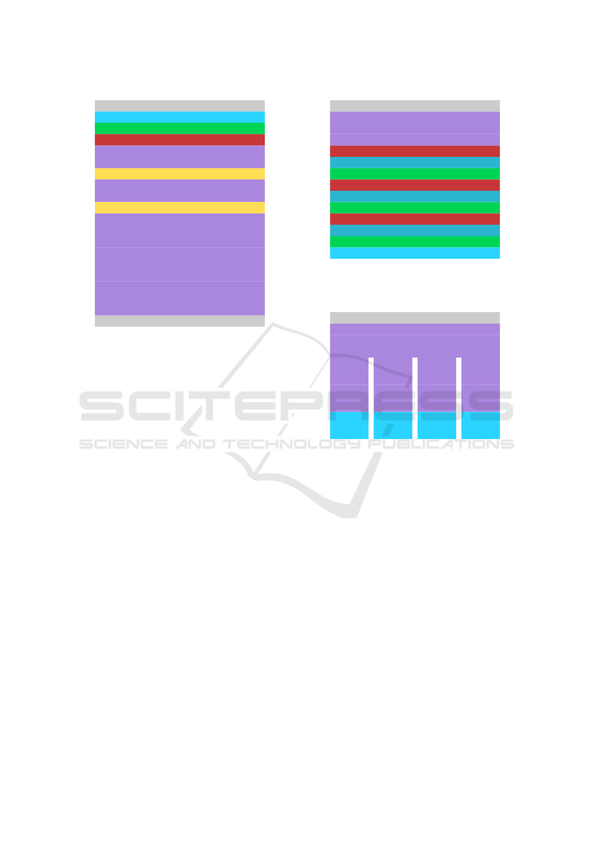
Input image

Conv. (7x7, 64 channels, stride 2)

ReLu

Batch Normalization

ResNet mod. (64 channels)

Maxpooling (2x2)

ResNet mod. (64 channels)

ResNet mod. (128 channels)

Maxpooling (2x2)

ResNet mod. (128 channels)

ResNet mod. (256 channels, 2x dilation)

ResNet mod. (512 channels, 4x dilation)

ResNet mod. (512 channels, 8x dilation)

ResNet mod. (512 channels, 4x dilation)

Backbone output

Figure 1: Structure of the proposed backbone for simul-

taneous semantic segmentation and object detection. The

ResNet modules have the same structure that is proposed in

(He et al., 2016) but use depthwise separable convolutions

to reduce the computational demand.

visualized in Figure 1. The ResNet modules have the

same structure that is proposed in (He et al., 2016).

But like Xception (Chollet, 2017), we use depthwise

separable convolutions to reduce the computational

demand.

The path for semantic segmentation has a convolu-

tional encoder-decoder structure. In the ﬁrst layers of

the encoder, the data tensor is sampled down by a fac-

tor of 8: The ﬁrst convolution has a stride of two and

there are two maxpooling layers that both downsam-

ple by a factor of two. This reduction of resolution

is necessary to decrease the computational demand of

the network. But after this reduction we use dilated

convolutions as proposed in (Chen et al., 2017). This

increases the receptive ﬁeld of the convolutions while

preserving spatial details and while keeping the num-

ber of learnable parameters constant.

The output of the backbone is then fed into mul-

tiple network heads. One head is the semantic seg-

mentation head. It is visualized in Figure 2. After

three more ResNet modules the data tensor is upsam-

pled again so that the ﬁnal segmentation map has the

same resolution as the input image. This is done us-

ing three transposed convolutions that each learn to

upsample by a factor of 2. An alternative would be

to upsample by a factor of 8 with just one transposed

convolution. But this way we can gradually reduce

the number of channels while increasing the spatial

Transposed Conv. (2x upsample, 128 channels)

ReLu

Batch Normalization

ResNet mod. (512 channels)

ReLu

Batch Normalization

ReLu

Batch Normalization

Conv. (1x1)

Transposed Conv. (2x upsample, 64 channels)

Transposed Conv. (2x upsample, 32 channels)

Backbone output

Figure 2: Structure of the network head for semantic seg-

mentation. The data tensor is upsampled by a factor of 8 to

compensate the downsampling in the backbone.

ResNet mod. (512 channels)

Conv.

(1x1)

ResNet

(128 ch.)

ResNet

(128 ch.)

Conv.

(1x1)

ResNet

(128 ch.)

ResNet

(128 ch.)

Conv.

(1x1)

ResNet

(512 ch.)

ResNet

(512 ch.)

Conv.

(1x1)

ResNet

(128 ch.)

ResNet

(128 ch.)

Backbone output

Figure 3: Structure of the network head for object detection.

The different outputs are an objectness score, a class score,

bounding box parameters regression and a feature embed-

ding per anchor box.

resolution. The ﬁnal convolution layer then reduces

the number of channels to the number of classes. Dur-

ing training, a softmax function is applied to its output

and it is trained using cross-entropy loss.

The second head of our proposed model is the

object detection head. It also takes the output of

the backbone as input and applies three more shared

ResNet modules. The output of the last shared ResNet

module is fed into four sub-networks of identical

structure but with a different number of channels.

Each consists of two more ResNet blocks and a ﬁnal

convolutional layer to adjust the number of channels

for the ﬁnal task.

The ﬁrst sub-network solves a binary classiﬁca-

tion problem. It predicts whether the corresponding

anchor box contains a relevant object or not. During

training, a softmax function is applied to its output.

Like RetinaNet (Lin et al., 2017) we use Focal Loss

to train this output. We chose α = 1.0 and γ = 2.0 as

Simultaneous Object Detection and Semantic Segmentation

557

Table 1: The parameters of our anchor boxes. At each lo-

cation of the feature map we generate anchor boxes for all

possible combinations of box ratio and box area.

Anchor box 0.25, 0.5, 1.0, 2.0, 4.0

ratios (w/h)

Anchor box 32, 48, 64, 96, 128, 192,

areas (in pixel) 256, 384, 512, 768, 1024,

1536, 2048, 3072, 4096,

6144, 8192, 12288, 16384,

24576, 32768, 49152, 65536,

98304, 131072, 196608,

262144, 393216, 524288

parameters.

The second sub-network also solves a classiﬁca-

tion problem. For all anchor boxes that contain a rel-

evant object it predicts its class. Like for the semantic

segmentation head, a softmax function is applied to

its output and it is trained using cross-entropy loss for

all active anchor boxes.

The third sub-network gives the regression output

of the bounding box parameters. These parameters

are the same as in R-CNN (Girshick et al., 2014). The

parameters for the used anchor boxes can be found in

Table 1. We generate anchor boxes at each location of

the feature map for all possible combinations of box

ratio and box area. Since we only downsample by a

factor of 8 in the encoder to preserve spatial details

for the semantic segmentation task we do not have

low-resolution feature maps. In contrast to RetinaNet

(Lin et al., 2017) we therefore only predict objects on

one feature map. In order to still be able to detect

objects of different sizes, we generate more anchor

boxes with different scales. We train the output with

smooth L1 loss for all active anchor boxes.

The fourth sub-network is optional. If desired it

can be used to learn a feature embedding for each de-

tected object. We include it here because it is use-

ful for some applications and we will use it in future

work. The feature embedding is trained using con-

trastive loss (Hadsell et al., 2006) for all active anchor

boxes. Since we train the network on single images

and not sequences all training examples come from

one image. We use all anchor boxes that correspond

to the same object as positive examples and all that

correspond to other objects as negative examples.

3.2 Training Procedure

We train our model on the Cityscapes dataset (Cordts

et al., 2016). It contains 5 000 ﬁnely annotated and

20 000 coarsely annotated training images. In order

to train the object detection head we extract bounding

boxes from the available instance labels. We do this

by taking the minimum and maximum of the x- and

y-coordinates of the instance polygons.

Our model is trained with the Adam optimizer

(Kingma and Ba, 2014). Like (Zhao et al., 2017), we

use a polynomial decay learning rate schedule of the

following form:

lr(iter) = base lr ·



iter

max iter



0.9

We use a batch size of 8 and a base learning rate of

0.001 and run the training for 300 000 iterations.

We use the approach proposed in (Kendall et al.,

2017) to weight the different losses of the multiple

tasks. However, we had to introduce soft limits to

make sure that the weights do not become too large or

too small. Our ﬁnal weighting formula therefore is:

loss

weighted,i

= exp(−s

) · loss

original,i

+ s

+ 1.5 · (1

u,i

) · s

u,i

−1

−

l,i

) · s

l,i

)

with s

l,i

= s

+ 10, s

u,i

= s

− 5

Here, s

are learnable parameters and 1(·) is the in-

dicator function. We reduced the learning rate for all

by a factor of 0.001 compared to all other weights.

These changes were necessary to keep the network

from diverging. One reason for this is that we do not

train bounding boxes for the coarsely annotated data.

If a lot of these training images are selected succes-

sively s

will be pushed to zero because the bounding

box loss is zero.

3.3 Bounding Box Target Generation

During training the target output of the neural network

for the bounding boxes is generated from the ground

truth bounding box list. Our procedure for this is as

follows: We initialize all anchor boxes as being “in-

active” (i. e. not corresponding to an object). Then

for each ground truth bounding box we calculate the

intersection over union with all anchor boxes. If the

IoU value is higher than 0.5 we set the anchor box to

being “active” and assign the class and regression pa-

rameters. If the IoU value is between 0.4 and 0.5 we

set the anchor box to “don’t care”. This ensures that

we do not get high losses and oscillating behavior for

anchor boxes right at the threshold.

There are a few corner cases that we also take

into account: If parts of the anchor box are outside

of the image but it contains an object we set it to

“don’t care”. We do this to avoid conﬂicting objec-

tives for the box regression task. If a ground truth

bounding box was not assigned to any anchor box (be-

cause there is none with an IoU higher than 0.5) but

ICPRAM 2020 - 9th International Conference on Pattern Recognition Applications and Methods

558

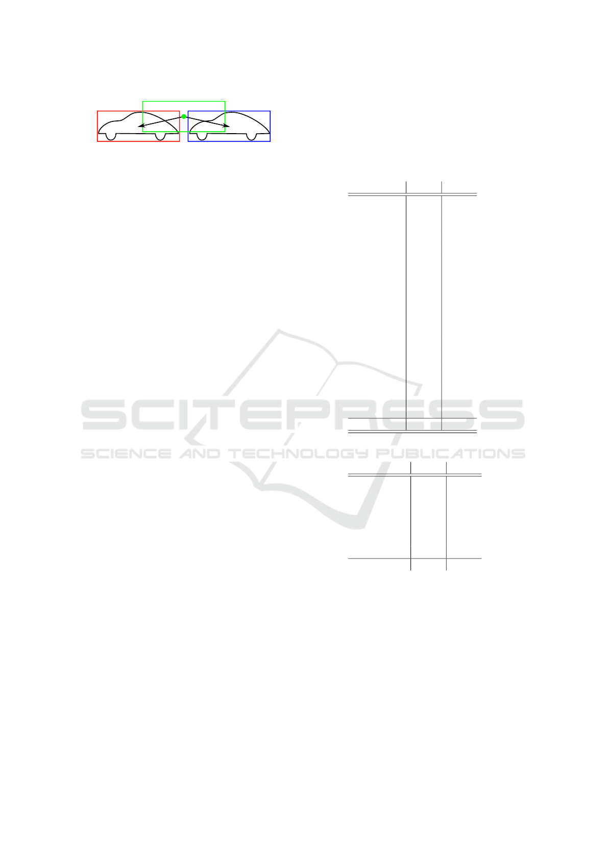
Figure 4: The green anchor box has high overlap with two

objects and would be “active” for both. Since both would

compete in the training objective for the box regression tar-

get the learned displacement would average out. There-

fore the decoded box would not align with any of the true

bounding boxes (red and blue) but would be in the middle.

We avoid this problem by setting these problematic anchor

boxes to “inactive” during training.

there is an anchor box with IoU higher than 0.4 we as-

sign it to this. This helps to also detect small objects

that fall between the grid. In case an anchor box can

be assigned to multiple ground truth bounding boxes

we choose the one with the highest IoU. But if the

absolute difference between the highest and the sec-

ond highest IoU value is less than 0.2 and both are

higher than 0.4 we set the anchor box to “inactive”.

This helps to ensure that objects are clearly separated.

We found that otherwise the regression output is just

the average of the displacements for all overlapping

objects. This means that the decoded bounding box

ends up being between the adjacent objects. It then is

too far away from all of them to be suppressed by the

non-maxima suppression. The problem is illustrated

in Figure 4.

4 EVALUATION

We train and evaluate our proposed neural network ar-

chitecture on the Cityscapes benchmark (Cordts et al.,

2016). The results for the semantic segmentation task

can be found in Table 2.

We evaluate the performance of our bounding box

detector for the “car” and “pedestrian” classes with

the ofﬁcial evaluation tool of the KITTI benchmark

(Geiger et al., 2012). The results can be found in Fig-

ure 5. Since we train the model with the Cityscapes

dataset we also want to evaluate on this dataset. It

however lacks annotations for the level of truncation

and occlusion. We therefore ignore these values dur-

ing the evaluation, making the task harder. But since

the images from the Cityscapes dataset have a higher

resolution than the ones from the KITTI dataset we

adjusted the size limits for the evaluation difﬁculty

levels. Here, we require a minimum width and height

of 10 for the “hard” difﬁculty level, 50 for the “mod-

erate” difﬁculty level and 100 for the “easy” difﬁculty

level. Because of these differences the results are

not comparable with the ones achieved on the KITTI

Table 2: Results of the semantic segmentation on the

Cityscapes validation dataset. The results have been com-

puted with the ofﬁcial evaluation script. The IoU metric is

the intersection-over-union metric used by PASCAL VOC

(Everingham et al., 2015). The iIoU metric is computed by

weighting each pixel with the ratio of the average instance

size and the size of the ground truth instance size.

Class IoU iIoU

road 0.963 -

sidewalk 0.736 -

building 0.868 -

wall 0.347 -

fence 0.385 -

pole 0.459 -

trafﬁc light 0.498 -

trafﬁc sign 0.625 -

vegetation 0.886 -

terrain 0.517 -

sky 0.905 -

person 0.711 0.518

rider 0.456 0.310

car 0.903 0.809

truck 0.381 0.212

bus 0.614 0.381

train 0.347 0.176

motorcycle 0.350 0.261

bicycle 0.653 0.462

Average 0.612 0.395

(a) Per-class results.

Category IoU iIoU

ﬂat 0.977 -

construction 0.872 -

object 0.530 -

nature 0.887 -

sky 0.905 -

human 0.721 0.543

vehicle 0.881 0.774

Average 0.825 0.658

(b) Per-category results.

dataset. But we hope that these are useful values that

can be used in future work for comparisons on the

Cityscapes dataset.

Especially the “car” class has many examples with

high occlusion levels in the Cityscapes dataset. This

explains the low recall in the “hard” difﬁculty level

for this class.

We also evaluate the object detection performance

on the KITTI dataset. Herw we follow the ofﬁcial

deﬁnitions of the difﬁculty levels from KITTI. The

results can be found in Figure 6. We randomly select

5 930 images from the KITTI training dataset to form

Simultaneous Object Detection and Semantic Segmentation

559

0.2

0.4

0.6

0.8

0 0.2 0.4 0.6 0.8 1

Precision

Recall

Car

Easy

Moderate

Hard

(a) Car class.

0.2

0.4

0.6

0.8

0 0.2 0.4 0.6 0.8 1

Precision

Recall

Pedestrian

Easy

Moderate

Hard

(b) Pedestrian class.

Class

Easy Moderate Hard

Car 84.5% 72.3% 50.9%

Pedestrian 70.9% 70.8% 56.5%

Figure 5: Results of the object detection on the Cityscapes

validation dataset. It uses the KITTI evaluation tool but with

an adjusted deﬁnition of the difﬁculty levels that is better

suited for Cityscapes.

0.2

0.4

0.6

0.8

0 0.2 0.4 0.6 0.8 1

Precision

Recall

Car

Easy

Moderate

Hard

(a) Car class.

0.2

0.4

0.6

0.8

0 0.2 0.4 0.6 0.8 1

Precision

Recall

Pedestrian

Easy

Moderate

Hard

(b) Pedestrian class.

Class Easy Moderate Hard

Car 82.1% 69.3% 60.2%

Pedestrian 79.5% 67.7% 60.1%

Figure 6: Results of the object detection on the KITTI vali-

dation dataset. Here we follow the ofﬁcial deﬁnition of the

difﬁculty levels.

a validation dataset. Then we mix the remaining im-

ages with the Cityscapes training images and ﬁne-tun

our model with that. One problem is that the gener-

ated bounding box labels from the Cityscapes dataset

and the labels from the KITTI dataset are not consis-

tent: While the generated bounding boxes cover only

the visible parts of each object the labels from the

KITTI dataset cover the projection of the whole ob-

ject. This explains the drop in precision for the “car”

class even for detection thresholds with low recall.

It also means that we observe lower recall at detec-

tion thresholds with low precision. Another issue is

that the images from the KITTI dataset have a lower

resolution while we tuned our model for the notably

higher resolution of the Cityscapes dataset. These re-

sults are therefore not directly comparable with a de-

tector that is only trained on the KITTI dataset. They

however give a lower bound for the expected perfor-

mance.

Our proposed architecture does not reach the level

of accuracy that is achieved by the best-performing

approaches on the Cityscapes and KITTI leader-

boards at the time of writing. It however gives good

accuracy while meeting the desired computation time

constraints. The inference time of the proposed con-

volutional neural network for images at the desired

resolution of 1 MP is 102 ms on an Nvidia Titan V

GPU. We measured this time using TensorFlow 1.13

and Nvidia TensorRT 5.1.2.2 RC at a precision of

16 bit.

5 CONCLUSION AND OUTLOOK

We demonstrate that two important vision tasks for

automated vehicles (semantic segmentation and ob-

ject detection) can be learned jointly by a single CNN.

We present a suitable neural network architecture for

this which takes the needs of both tasks into account.

It does not achieve the level of accuracy that the

the best-performing models offer today. However, it

gives good accuracy while meeting the run-time con-

straints of the application: Our approach achieves the

design goal of a framerate of 10 Hz on 1 MP images.

We currently use the presented approach in our re-

search vehicle. The semantic segmentation gives in-

formation about the static and dynamic parts of the

world. This information is useful for mapping where

we only want to map the static parts. It can also be

used for mapless driving or freespace validation. The

object detections are fused with detections from other

sensors and then used by the behavior and trajectory

planning modules.

We will focus on further reducing the run-time of

our object detection head without losing accuracy. In

future work we will present a tracking approach for

road users that is based on this work.

REFERENCES

Badrinarayanan, V., Kendall, A., and Cipolla, R. (2017).

SegNet: A Deep Convolutional Encoder-Decoder Ar-

chitecture for Image Segmentation. IEEE Transac-

tions on Pattern Analysis and Machine Intelligence.

Baxter, J. (2000). A Model of Inductive Bias Learning.

Journal of Artiﬁcial Intelligence Research.

Chen, L.-C., Papandreou, G., Schroff, F., and Adam, H.

(2017). Rethinking Atrous Convolution for Semantic

Image Segmentation.

ICPRAM 2020 - 9th International Conference on Pattern Recognition Applications and Methods

560

Chen, L.-C., Zhu, Y., Papandreou, G., Schroff, F., and

Adam, H. (2018). Encoder-Decoder with Atrous Sep-

arable Convolution for Semantic Image Segmentation.

In Proceedings of the European Conference on Com-

puter Vision (ECCV).

Chollet, F. (2017). Xception: Deep Learning with Depth-

wise Separable Convolutions. In Proceedings of the

IEEE Conference on Computer Vision and Pattern

Recognition.

Cordts, M., Omran, M., Ramos, S., Rehfeld, T., Enzweiler,

M., Benenson, R., Franke, U., Roth, S., and Schiele,

B. (2016). The Cityscapes Dataset for Semantic Ur-

ban Scene Understanding. In Proc. of the IEEE Con-

ference on Computer Vision and Pattern Recognition

(CVPR).

Everingham, M., Eslami, S. A., Van Gool, L., Williams,

C. K., Winn, J., and Zisserman, A. (2015). The Pas-

cal Visual Object Classes Challenge: A Retrospective.

International Journal of Computer Vision.

Geiger, A., Lenz, P., and Urtasun, R. (2012). Are we ready

for Autonomous Driving? The KITTI Vision Bench-

mark Suite. In Conference on Computer Vision and

Pattern Recognition (CVPR).

Girshick, R. (2015). Fast R-CNN. In Proceedings of the

IEEE Conference on Computer Vision and Pattern

Recognition.

Girshick, R., Donahue, J., Darrell, T., and Malik, J. (2014).

Rich feature hierarchies for accurate object detection

and semantic segmentation. In Proceedings of the

IEEE Conference on Computer Vision and Pattern

Recognition.

Hadsell, R., Chopra, S., and LeCun, Y. (2006). Dimension-

ality Reduction by Learning an Invariant Mapping. In

Proceedings of the IEEE Conference on Computer Vi-

sion and Pattern Recognition.

He, K., Zhang, X., Ren, S., and Sun, J. (2016). Identity

Mappings in Deep Residual Networks. In European

Conference on Computer Vision.

Kendall, A., Gal, Y., and Cipolla, R. (2017). Multi-

Task Learning Using Uncertainty to Weigh Losses for

Scene Geometry and Semantics. CoRR.

Kingma, D. P. and Ba, J. (2014). Adam: A Method for

Stochastic Optimization.

Lin, T.-Y., Goyal, P., Girshick, R. B., He, K., and Doll

ar,

P. (2017). Focal Loss for Dense Object Detection. In

ICCV. IEEE Computer Society.

Liu, W., Anguelov, D., Erhan, D., Szegedy, C., Reed, S.,

Fu, C.-Y., and Berg, A. C. (2016). SSD: Single Shot

MultiBox Detector. In European Conference on Com-

puterVision.

Long, J., Shelhamer, E., and Darrell, T. (2015). Fully Con-

volutional Networks for Semantic Segmentation. In

Proceedings of the IEEE Conference on Computer Vi-

sion and Pattern Recognition.

Meyer, A., Salscheider, N. O., Orzechowski, P., and Stiller,

C. (2018). Deep Semantic Lane Segmentation for

Mapless Driving.

Redmon, J., Divvala, S., Girshick, R., and Farhadi, A.

(2016). You Only Look Once: Uniﬁed, Real-Time

Object Detection. In Proceedings of the IEEE Confer-

ence on Computer Vision and Pattern Recognition.

Redmon, J. and Farhadi, A. (2017). YOLO9000: Better,

Faster, Stronger. In Proceedings of the IEEE Confer-

ence on Computer Vision and Pattern Recognition.

Redmon, J. and Farhadi, A. (2018). YOLOv3: An Incre-

mental Improvement.

Ren, S., He, K., Girshick, R. B., and Sun, J. (2015). Faster

R-CNN: Towards Real-Time Object Detection with

Region Proposal Networks. CoRR.

Sistu, G., Leang, I., and Yogamani, S. (2019). Real-time

Joint Object Detection and Semantic Segmentation

Network for Automated Driving.

Teichmann, M., Weber, M., Zoellner, M., Cipolla, R., and

Urtasun, R. (2018). MultiNet: Real-time Joint Seman-

tic Reasoning for Autonomous Driving. In 2018 IEEE

Intelligent Vehicles Symposium (IV).

Uhrig, J., Cordts, M., Franke, U., and Brox, T.

(2016). Pixel-Level Encoding and Depth Layering for

Instance-Level Semantic Labeling. In GCPR.

van de Sande, K. E. A., Uijlings, J. R. R., Gevers, T., and

Smeulders, A. W. M. (2011). Segmentation as Selec-

tive Search for Object Recognition. In ICCV.

Wu, Z., Shen, C., and van den Hengel, A. (2016). Wider

or Deeper: Revisiting the ResNet Model for Visual

Recognition.

Zhao, H., Shi, J., Qi, X., Wang, X., and Jia, J. (2017). Pyra-

mid Scene Parsing Network. In CVPR. IEEE Com-

puter Society.

Simultaneous Object Detection and Semantic Segmentation

561