ConvPoseCNN: Dense Convolutional 6D Object Pose Estimation

Catherine Capellen, Max Schwarz

and Sven Behnke

Autonomous Intelligent Systems Group of University of Bonn, Germany

Keywords:

Pose Estimation, Dense Prediction, Deep Learning.

Abstract:

6D object pose estimation is a prerequisite for many applications. In recent years, monocular pose estimation

has attracted much research interest because it does not need depth measurements. In this work, we introduce

ConvPoseCNN, a fully convolutional architecture that avoids cutting out individual objects. Instead we pro-

pose pixel-wise, dense prediction of both translation and orientation components of the object pose, where the

dense orientation is represented in Quaternion form. We present different approaches for aggregation of the

dense orientation predictions, including averaging and clustering schemes. We evaluate ConvPoseCNN on the

challenging YCB-Video Dataset, where we show that the approach has far fewer parameters and trains faster

than comparable methods without sacriﬁcing accuracy. Furthermore, our results indicate that the dense orien-

tation prediction implicitly learns to attend to trustworthy, occlusion-free, and feature-rich object regions.

1 INTRODUCTION

Given images of known, rigid objects, 6D object pose

estimation describes the problem of determining the

identity of the objects, their position and their orienta-

tion. Recent research focuses on increasingly difﬁcult

datasets with multiple objects per image, cluttered en-

vironments, and partially occluded objects. Symmet-

ric objects pose a particular challenge for orientation

estimation, because multiple solutions or manifolds

of solutions exist. While the pose problem mainly

receives attention from the computer vision commu-

nity, in recent years there have been multiple robotics

competitions involving 6D pose estimation as a key

component, for example the Amazon Picking Chal-

lenge of 2015 and 2016 and the Amazon Robotics

Challenge of 2017, where robots had to pick objects

from highly cluttered bins. The pose estimation prob-

lem is also highly relevant in human-designed, less

structured environments, e.g. as encountered in the

RoboCup@Home competition Iocchi et al. (2015),

where robots have to operate within home environ-

ments.

https://orcid.org/0000-0002-9942-6604

https://orcid.org/0000-0002-5040-7525

2 RELATED WORK

For a long time, feature-based and template-based

methods were popular for 6D object pose estima-

tion (Lowe, 2004; Wagner et al., 2008; Hinterstoisser

et al., 2012a,b). However, feature-based methods

rely on distinguishable features and perform badly

for texture-poor objects. Template-based methods do

not work well if objects are partially occluded. With

deep learning methods showing success for different

image-related problem settings, models inspired or

extending these have been used increasingly. Many

methods use established architectures to solve sub-

problems, as for example semantic segmentation or

instance segmentation. Apart from that, most re-

cent methods use deep learning for their complete

pipeline. We divide these methods into two groups:

Direct pose regression methods (Do et al., 2018; Xi-

ang et al., 2018) and methods that predict 2D-3D ob-

ject correspondences and then solve the PnP problem

to recover the 6D pose. The latter can be further di-

vided into methods that predict dense, pixel-wise cor-

respondences (Brachmann et al., 2014, 2016; Krull

et al., 2015) and, more recently, methods that esti-

mate the 2D coordinates of selected keypoints, usu-

ally the 3D object bounding box corners (Oberweger

et al., 2018; Rad and Lepetit, 2017; Tekin et al., 2018;

Tremblay et al., 2018).

Oberweger et al. (2018) predict the projection of

the 3D bounding box as a heat map. To achieve ro-

162

Capellen, C., Schwarz, M. and Behnke, S.

ConvPoseCNN: Dense Convolutional 6D Object Pose Estimation.

DOI: 10.5220/0008990901620172

In Proceedings of the 15th International Joint Conference on Computer Vision, Imaging and Computer Graphics Theory and Applications (VISIGRAPP 2020) - Volume 5: VISAPP, pages

162-172

ISBN: 978-989-758-402-2; ISSN: 2184-4321

Figure 1: Dense Prediction of 6D pose parameters inside

ConvPoseCNN. The dense predictions are aggregated on

the object level to form 6D pose outputs.

bustness to occlusion, they predict the heat map inde-

pendently for small object patches before adding them

together. The maximum is selected as the corner posi-

tion. If patches are ambiguous, the training technique

implicitly results in an ambiguous heat map predic-

tion. This method also uses Feature Mapping (Rad

et al., 2018), a technique to bridge the domain-gap

between synthetic and real training data.

We note that newer approaches increasingly focus

on the monocular pose estimation problem without

depth information (Brachmann et al., 2016; Do et al.,

2018; Jafari et al., 2017; Rad and Lepetit, 2017; Ober-

weger et al., 2018; Tekin et al., 2018; Tremblay et al.,

2018; Xiang et al., 2018). In addition to predicting

the pose from RGB or RGB-D data, there are several

reﬁnement techniques for pose improvement after the

initial estimation. Li et al. (2018) introduce a render-

and-compare technique that improves the estimation

only using the original RGB input. If depth is avail-

able, ICP registration can be used to reﬁne poses.

As a representative of the direct regression

method, we discuss PoseCNN (Xiang et al., 2018)

in more detail. It delivered state-of-the-art perfor-

mance on the occluded LINEMOD dataset and in-

troduced a more challenging dataset, the YCB-Video

Dataset. PoseCNN decouples the problem of pose

estimation into estimating the translation and orien-

tation separately. A pretrained VGG16 backbone is

used for feature extraction. The features are processed

in three different branches: Two fully convolutional

branches estimate a semantic segmentation, center di-

rections, and the depth for every pixel of the image.

The third branch consists of a RoI pooling and a fully-

connected architecture which regresses to a quater-

nion describing the rotation for each region of inter-

est.

RoI pooling – i.e. cutting out and size normaliz-

ing an object hypothesis – was originally developed

for the object detection problem (Girshick, 2015),

where it is used to extract an object-centered and

size-normalized view of the extracted CNN features.

The following classiﬁcation network, usually consist-

ing of a few convolutional and fully-connected layers,

then directly computes class scores for the extracted

region. As RoI pooling focusses on individual object

hypotheses, it looses contextual information, which

might be important in cluttered scenes where objects

are densely packed and occlude each other. RoI pool-

ing requires random access to the source feature map

for cutting out and interpolating features. Such ran-

dom access patterns are expensive to implement in

hardware circuits and have no equivalent in the visual

cortex (Kandel et al., 2000). Additionally, RoI pool-

ing is often followed by fully connected layers, which

drive up parameter count and inference/training time.

Following the initial breakthroughs using RoI

pooling, simpler architectures for object detection

have been proposed which compute the class scores

in a fully convolutional way (Redmon et al., 2016).

An important insight here is that a CNN is essen-

tially equivalent to a sliding-window operator, i.e.

fully-convolutional classiﬁcation is equivalent to RoI-

pooled classiﬁcation with a ﬁxed region size. While

the in-built size-invariance of RoI pooling is lost,

fully-convolutional architectures typically outperform

RoI-based ones in terms of model size and train-

ing/inference speed. With a suitably chosen loss func-

tion that addresses the inherent example imbalances

during training (Lin et al., 2017), fully-convolutional

architectures reach state-of-the-art accuracy in object

detection.

Following this idea, we developed a fully-

convolutional architecture evolved from PoseCNN,

that replaces the RoI pooling-based orientation esti-

mation of PoseCNN with a fully-convolutional, pixel-

wise quaternion orientation prediction (see Fig. 1).

Recently, Peng et al. (2019) also removed the RoI-

pooled orientation prediction branch, but with a dif-

ferent method: Here, 2D directions to a ﬁxed num-

ber of keypoints are densely predicted. Each key-

point is found using a separate Hough transform and

the pose is then estimated using a PnP solver utiliz-

ing the known keypoint correspondences. In con-

trast, our method retains the direct orientation regres-

sion branch, which may be interesting in resource-

constrained scenarios, where the added overhead of

additional Hough transforms and PnP solving is un-

desirable.

Our proposed changes unify the architecture and

make it more parallel: PoseCNN ﬁrst predicts the

translation and the regions of interest (RoI) and then,

sequentially for each RoI estimates object orientation.

Our architecture can perform the rotation estimation

for multiple objects in parallel, independent from the

translation estimation. We investigated different av-

ConvPoseCNN: Dense Convolutional 6D Object Pose Estimation

163

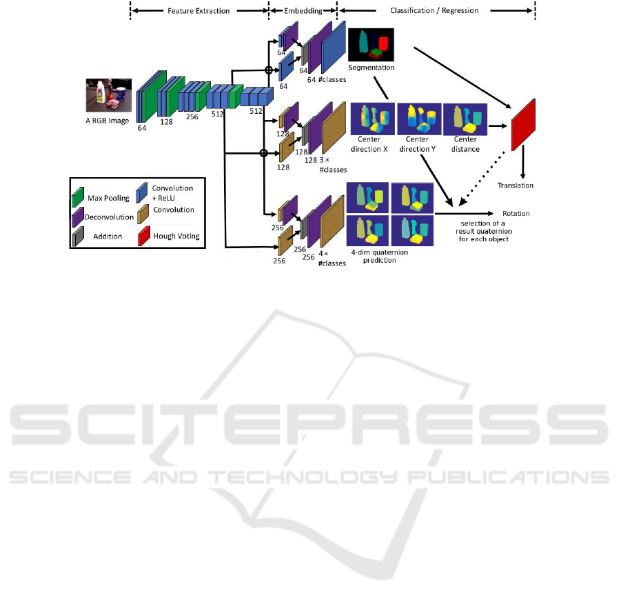
Figure 2: Our ConvPoseCNN architecture for convolutional pose estimation. During aggregation, candidate quaternions are

selected according to the semantic segmentation results or according to Hough inlier information. Figure adapted from (Xiang

et al., 2018).

eraging and clustering schemes for obtaining a ﬁnal

orientation from our pixel-wise estimation. We com-

pare the results of our architecture to PoseCNN on the

YCB-Video Dataset (Xiang et al., 2018). We show

that our fully-convolutional architecture with pixel-

wise prediction achieves precise results while using

far less parameters. The simpler architecture also re-

sults in shorter training times.

In summary, our contributions include:

1. A conceptually simple, small, and fast-to-train ar-

chitecture for dense orientation estimation, whose

prediction is easily interpretable due to its dense

nature,

2. a comparison of different orientation aggregation

techniques, and

3. a thorough evaluation and ablation study of the

different design choices on the challenging YCB-

Video dataset.

3 METHOD

We propose an architecture derived from PoseCNN

(Xiang et al., 2018), which predicts, starting from

RGB images, 6D poses for each object in the im-

age. The network starts with the convolutional back-

bone of VGG16 (Simonyan and Zisserman, 2014)

that extracts features. These are subsequently pro-

cessed in three branches: The fully-convolutional seg-

mentation branch that predicts a pixel-wise semantic

segmentation, the fully-convolutional vertex branch,

which predicts a pixel-wise estimation of the center

direction and center depth, and the quaternion esti-

mation branch. The segmentation and vertex branch

results are combined to vote for object centers in a

Hough transform layer. The Hough layer also predicts

bounding boxes for the detected objects. PoseCNN

then uses these bounding boxes to crop and pool the

extracted features which are then fed into a fully-

connected neural network architecture. This fully-

connected part predicts an orientation quaternion for

each bounding box.

Our architecture, shown in Fig. 2, replaces the

quaternion estimation branch of PoseCNN with a

fully-convolutional architecture, similar to the seg-

mentation and vertex prediction branch. It predicts

quaternions pixel-wise. We call it ConvPoseCNN

(short for convolutional PoseCNN). Similarly to

PoseCNN, quaternions are regressed directly using

a linear output layer. The added layers have the

same architectural parameters as in the segmenta-

tion branch (ﬁlter size 3×3) and are thus quite light-

weight.

While densely predicting orientations at the pixel

level might seem counter-intuitive, since orientation

estimation typically needs long-range information

from distant pixels, we argue that due to the total

depth of the convolutional network and the involved

pooling operations the receptive ﬁeld for a single out-

put pixel covers large parts of the image and thus al-

lows long-range information to be considered during

orientation prediction.

VISAPP 2020 - 15th International Conference on Computer Vision Theory and Applications

164

3.1 Aggregation of Dense Orientation

Predictions

We estimate quaternions pixel-wise and use the pre-

dicted segmentation to identify which quaternions be-

long to which object. If multiple instances of one ob-

ject can occur, one could use the Hough inliers instead

of the segmentation. Before the aggregation of the se-

lected quaternions to a ﬁnal orientation estimate, we

ensure that each predicted quaternion q corresponds

to a rotation by scaling it to unit norm. However, we

found that the norm w = ||q|| prior to scaling is of in-

terest for aggregation: In feature-rich regions, where

there is more evidence for the orientation prediction,

it tends to be higher (see Section 4.8). We investigated

averaging and clustering techniques for aggregation,

optionally weighted by w.

For averaging the predictions we use the weighted

quaternion average as deﬁned by Markley et al.

(2007). Here, the average ¯q of quaternion samples

, ..., q

with weights w

, ..., w

is deﬁned using the

corresponding rotation matrices R(q

), ..., R(q

¯q = arg min

q∈S

∑

i=1

||R(q) −R(q

)||

, (1)

where S

is the unit 3-sphere and || · ||

is the Frobe-

nius norm. This deﬁnition avoids any problems aris-

ing from the antipodal symmetry of the quaternion

representation. The exact solution to the optimiza-

tion problem can be found by solving an eigenvalue

problem (Markley et al., 2007).

For the alternative clustering aggregation, we fol-

low a weighted RANSAC scheme: For quaternions

Q = {q

, ..., q

} and their weights w

, ..., w

associ-

ated with one object this algorithm repeatedly chooses

a random quaternion ˆq ∈ Q with a probability propor-

tional to its weight and then determines the inlier set

Q = {q ∈ Q|d(q, ˆq) < t}, where d(·, ·) is the angular

distance. Finally, the ˆq with largest

∑

∈

is se-

lected as the result quaternion.

The possibility of weighting the individual sam-

ples is highly useful in this context, since we expect

that parts of the object are more important for deter-

mining the correct orientation than others (e.g. the

handle of a cup). In our architecture, sources of such

pixel-wise weight information can be the segmenta-

tion branch with the class conﬁdence scores, as well

as the predicted quaternion norms ||q

||, ..., ||q

|| be-

fore normalization.

3.2 Losses and Training

For training the orientation branch, Xiang et al.

(2018) propose the ShapeMatch loss. This loss cal-

culates a distance measure between point clouds of

the object rotated by quaternions ˜q and q:

SMLoss( ˜q, q) =

(

SLoss( ˜q, q) if symmetric,

PLoss( ˜q, q) otherwise.

(2)

Given a set of 3D points M, where m = |M| and

R(q) and R( ˜q) are the rotation matrices correspond-

ing to ground truth and estimated quaternion, respec-

tively, and PLoss and SLoss are deﬁned in (Xiang

et al., 2018) as follows:

PLoss( ˜q, q) =

∑

x∈M

||R( ˜q)x − R(q)x||

, (3)

SLoss( ˜q, q) =

∑

∈M

min

∈M

||R( ˜q)x

− R(q)x

(4)

Similar to the ICP objective, SLoss does not penalize

rotations of symmetric objects that lead to equivalent

shapes.

In our case, ConvPoseCNN outputs a dense, pixel-

wise orientation prediction. Computing the SMLoss

pixel-wise is computationally prohibitive. First ag-

gregating the dense predictions and then calculating

the orientation loss makes it possible to train with

SMLoss. In this setting, we use a naive average, the

normalized sum of all quaternions, to facilitate back-

propagation through the aggregation step. As a more

efﬁcient alternative we experiment with pixel-wise L2

or QLoss (Billings and Johnson-Roberson, 2018) loss

functions, that are evaluated for the pixels indicated

by the ground-truth segmentation. QLoss is designed

to handle the quaternion symmetry. For two quater-

nions ¯q and q it is deﬁned as:

QLoss( ¯q, q) = log(ε + 1 − | ¯q · q|), (5)

where ε is introduced for stability.

The ﬁnal loss function used during training is,

similarly to PoseCNN, a linear combination of seg-

mentation (L

seg

), translation (L

trans

), and orientation

loss (L

rot

L = α

seg

+ α

trans

+ α

rot

. (6)

Values for the α coefﬁcients as used in our exper-

iments are given in Section 4.4.

4 EVALUATION

4.1 Datasets

We perform our experiments on the challenging

YCB-Video Dataset (Xiang et al., 2018). The dataset

ConvPoseCNN: Dense Convolutional 6D Object Pose Estimation

165

contains 133,936 images extracted from 92 videos,

showing 21 rigid objects. For each object the dataset

contains a point model with 2620 points each and a

mesh ﬁle. Additionally the dataset contains 80.000

synthetic images. The synthetic images are not phys-

ically realistic. Randomly selected images from

SUN2012 (Xiao et al., 2010) and ObjectNet3D (Xi-

ang et al., 2016) are used as backgrounds for the syn-

thetic frames.

When creating the dataset only the ﬁrst frame of

each video was annotated manually and the rest of

the frames were inferred using RGB-D SLAM tech-

niques. Therefore, the annotations are sometimes less

precise.

The images contain multiple relevant objects in

each image, as well as occasionally uninteresting ob-

jects and distracting background. Each object appears

at most once in each image. The dataset includes sym-

metric and texture-poor objects, which are especially

challenging.

4.2 Evaluation Metrics

We evaluate our method under the AUC P and AUC S

metrics as deﬁned for PoseCNN (Xiang et al., 2018).

For each model we report the total area under the

curve for all objects in the test set. The AUC P variant

is based on a point-wise distance metric which does

not consider symmetry effects (also called ADD). In

contrast, AUC S is based on an ICP-like distance

function (also called ADD-S) which is robust against

symmetry effects. For details, we refer to (Xiang

et al., 2018). We additionally report the same met-

ric when the translation is not applied, referred to as

“rotation only”.

4.3 Implementation

We implemented our experiments using the PyTorch

framework (Paszke et al., 2017), with the Hough vot-

ing layer implemented on CPU using Numba (Lam

et al., 2015), which proved to be more performant

than a GPU implementation. Note that there is no

backpropagation through the Hough layer.

For the parts that are equivalent to PoseCNN we

followed the published code, which has some differ-

ences to the corresponding publication (Xiang et al.,

2018), including the application of dropout and esti-

mation of log(z) instead of z in the translation branch.

We found that these design choices improve the re-

sults in our architecture as well.

Table 1: Weighting strategies for ConvPoseCNN L2.

Method 6D pose

Rotation only

AUC P AUC S AUC P AUC S

PoseCNN

53.71 76.12 78.87 93.16

unit weights 56.59 78.86 72.87 90.68

norm weights 57.13 79.01 73.84 91.02

segm. weights 56.63 78.87 72.95 90.71

Following Xiang et al. (2018)

Calculated from the PoseCNN model published in the YCB-

Video Toolbox.

4.4 Training

For training ConvPoseCNN we generally follow the

same approach as for PoseCNN: We use SGD with

learning rate 0.001 and momentum 0.9. For the over-

all loss we use α

seg

= α

trans

= 1. For the L2 and

the QLoss we use also α

rot

= 1, for the SMLoss we

used α

rot

= 100. To bring the depth error to a sim-

ilar range as the center direction error, we scale the

(metric) depth by a factor of 100.

We trained our network with a batch size of 2 for

approximately 300,000 iterations utilizing the early

stopping technique. Since the YCB-Video Dataset

contains real and synthetic frames, we choose a syn-

thetic image with a probability of 80% and render it

onto a random background image from the SUN2012

(Xiao et al., 2010) and ObjectNet3D (Xiang et al.,

2016) dataset.

4.5 Prediction Averaging

We ﬁrst evaluated the different orientation loss func-

tions presented in Section 3.2: L2, QLoss, and SM-

Loss. For SMLoss, we ﬁrst averaged the quaternions

predicted for each object with a naive average before

calculating the loss.

The next pipeline stage after predicting dense ori-

entation is the aggregation into a single orientation.

We ﬁrst investigated the quaternion average follow-

ing (Markley et al., 2007), using either segmentation

conﬁdence or quaternion norm as sample weights. As

can be seen in Table 1, norm weighting showed the

best results.

Since weighting seemed to be beneﬁcial, which

suggests that there are less precise or outlier predic-

tions that should be ignored, we experimented with

pruning of the predictions using the following strat-

egy: The quaternions are sorted by conﬁdence and

the least conﬁdent ones, according to a removal frac-

tion 0 ≤ λ ≤ 1 are discarded. The weighted average

of the remaining quaternions is then computed as de-

scribed above. The results are shown as pruned(λ)

VISAPP 2020 - 15th International Conference on Computer Vision Theory and Applications

166

Table 2: Quaternion pruning for ConvPoseCNN L2.

Method 6D pose

Rotation only

AUC P AUC S AUC P AUC S

PoseCNN 53.71 76.12 78.87 93.16

pruned(0) 57.13 79.01 73.84 91.02

pruned(0.5) 57.43 79.14 74.43 91.33

pruned(0.75) 57.43 79.19 74.48 91.45

pruned(0.9) 57.37 79.23 74.41 91.50

pruned(0.95) 57.39 79.21 74.45 91.50

single 57.11 79.22 74.00 91.46

Following Xiang et al. (2018).

Table 3: Clustering strategies for ConvPoseCNN L2.

Method 6D pose Rotation only

AUC P AUC S AUC P AUC S

PoseCNN 53.71 76.12 78.87 93.16

RANSAC(0.1) 57.18 79.16 74.12 91.37

RANSAC(0.2) 57.36 79.20 74.40 91.45

RANSAC(0.3) 57.27 79.20 74.13 91.35

RANSAC(0.4) 57.00 79.13 73.55 91.14

W-RANSAC(0.1) 57.27 79.20 74.29 91.45

W-RANSAC(0.2) 57.42 79.26 74.53 91.56

W-RANSAC(0.3) 57.38 79.24 74.36 91.46

pruned(0.75) 57.43 79.19 74.48 91.45

most conﬁdent 57.11 79.22 74.00 91.46

RANSAC uses unit weights, while W-RANSAC is weighted by

quaternion norm. PoseCNN and the best performing averaging

methods are shown for comparison. Numbers in parentheses de-

scribe the clustering threshold in radians.

in Table 2. We also report the extreme case, where

only the most conﬁdent quaternion is left. Overall,

pruning shows a small improvement, with the ideal

value of λ depending on the target application. More

detailed evaluation shows that especially the symmet-

ric objects show a clear improvement when pruning.

We attribute this to the fact that the averaging meth-

ods do not handle symmetries, i.e. an average of two

shape-equivalent orientations can be non-equivalent.

Pruning might help to reduce other shape-equivalent

but L2-distant predictions and thus improves the ﬁnal

prediction.

4.6 Prediction Clustering

For clustering with the RANSAC strategies, we used

the angular distance between rotations as the clus-

tering distance function and performed 50 RANSAC

iterations. In contrast to the L2 distance in quater-

nion space, this distance function does not suffer from

the antipodal symmetry of the quaternion orienta-

tion representation. The results for ConvPoseCNN

L2 are shown in Table 3. For comparison the best-

performing averaging strategies are also listed. The

weighted RANSAC variant performs generally a bit

better than the non-weighted variant for the same

inlier thresholds, which correlates to our ﬁndings

in Section 4.5. In comparison, clustering performs

slightly worse than the averaging strategies for AUC

P, but slightly better for AUC S—as expected due to

the symmetry effects.

4.7 Loss Variants

The aggregation methods showed very similar results

for the QLoss trained model, which are omitted here

for brevity. For the SMLoss variant, we report the

results in Table 5. Norm weighting improves the re-

sult, but pruning does not. This suggests that there are

less-conﬁdent but important predictions with higher

distance from the mean, so that their removal signif-

icantly affects the average. This could be an effect

of training with the average quaternion, where such

behavior is not discouraged. The RANSAC cluster-

ing methods generally produce worse results than the

averaging methods in this case. We conclude that the

average-before-loss scheme is not advantageous and a

fast dense version of SMLoss would need to be found

in order to apply it in our architecture. The pixel-wise

losses obtain superior performance.

4.8 Final Results

Figure 3 shows qualitative results of our best-

performing model on the YCB-Video dataset. We es-

pecially note the spatial structure of our novel dense

orientation estimation. Due to the dense nature, its

output is strongly correlated to image location, which

allows straightforward visualization and analysis of

the prediction error w.r.t. the involved object shapes.

As expected, regions that are close to boundaries be-

tween objects or far away from orientation-deﬁning

features tend to have higher prediction error. How-

ever, this is nicely compensated by our weighting

scheme, as the predicted quaternion norm || ˜q|| before

normalization correlates with this effect, i.e. is lower

in these regions. We hypothesize that this is an im-

plicit effect of the dense loss function: In areas with

high certainty (i.e. easy to recognize), the network

output is encouraged strongly in one direction. In ar-

eas with low certainty (i.e. easy to confuse), the net-

work cannot sufﬁciently discriminate and gets pulled

into several directions, resulting in outputs close to

zero.

In Table 4, we report evaluation metrics for our

models with the best averaging or clustering method.

As a baseline, we include the PoseCNN results, com-

ConvPoseCNN: Dense Convolutional 6D Object Pose Estimation

167

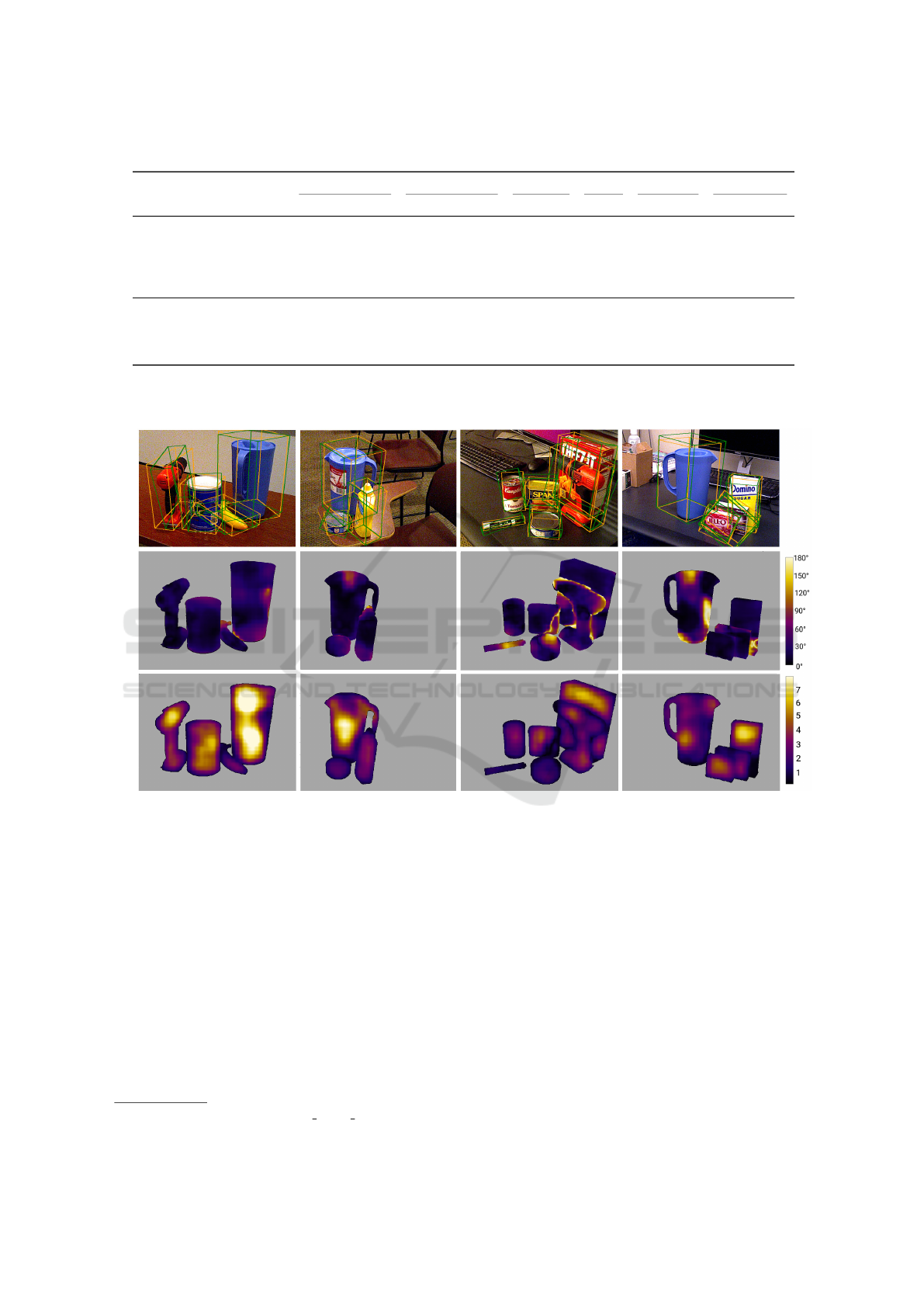
Table 4: 6D pose, translation, rotation, and segmentation results.

6D pose Rotation only NonSymC SymC Translation Segmentation

AUC P AUC S AUC P AUC S AUC P AUC S Error [m] IoU

full network

PoseCNN 53.71 76.12 78.87 93.16 60.49 63.28 0.0520 0.8369

PoseCNN (own impl.) 53.29 78.31 69.00 90.49 60.91 57.91 0.0465 0.8071

ConvPoseCNN QLoss 57.16 77.08 80.51 93.35 64.75 53.95 0.0565 0.7725

ConvPoseCNN Shape 55.54 79.27 72.15 91.55 62.77 56.42 0.0455 0.8038

ConvPoseCNN L2 57.42 79.26 74.53 91.56 63.48 58.85 0.0411 0.8044

GT segm.

PoseCNN (own impl.) 52.90 80.11 69.60 91.63 76.63 84.15 0.0345 1

ConvPoseCNN QLoss 57.73 79.04 81.20 94.52 88.27 90.14 0.0386 1

ConvPoseCNN Shape 56.27 81.27 72.53 92.27 77.32 89.06 0.0316 1

ConvPoseCNN L2 59.50 81.54 76.37 92.32 80.67 85.52 0.0314 1

The average translation error, the segmentation IoU and the AUC metrics for different models. The AUC results were achieved us-

ing weighted RANSAC(0.1) for ConvPoseCNN QLoss, Markley’s norm weighted average for ConvPoseCNN Shape and weighted

RANSAC(0.2) for ConvPoseCNN L2. GT segm. refers to ground truth segmentation (i.e. only pose estimation).

Input + PredictionOrientation ErrorPrediction Norm || ˜q||

Figure 3: Qualitative results from ConvPoseCNN L2 on the YCB-Video test set. Top: The orange boxes show the ground

truth bounding boxes, the green boxes the 6D pose prediction. Middle: Angular error of the dense quaternion prediction ˜q

w.r.t. ground truth, masked by ground truth segmentation. Bottom: Quaternion prediction norm || ˜q|| before normalization.

This measure is used for weighted aggregation. Note that the prediction norm is low in high-error regions and high in regions

that are far from occlusions and feature-rich.

puted from the YCB-Video Toolbox model

. We

also include our re-implementation of PoseCNN. We

achieved similar ﬁnal AUCs on the test set. We also

show more detailed results with regard to translation

and segmentation of the different models. For this we

report the average translation error and the segmen-

tation IoU for all models in Table 4. They show that

there is a strong inﬂuence of the translation estimation

on the AUC losses. However, for the models with bet-

ter translation estimation, the orientation estimation is

worse.

https://github.com/yuxng/YCB Video toolbox

For the total as reported by PoseCNN, all

three ConvPoseCNNs have a bit higher AUC than

PoseCNN, but only the model trained with QLoss has

a similar orientation estimation to PoseCNN. Com-

pared to PoseCNN, some models perform better for

the orientation and some better for the translation

even though the translation estimation branch is the

same for all of these networks. We were interested in

the models performance with regard to the symmetric

and non-symmetric objects. For this we calculated the

class-wise average over the AUCs for the symmetric

and non-symmetric objects separately. In Table 4 we

VISAPP 2020 - 15th International Conference on Computer Vision Theory and Applications

168

Table 5: Results for ConvPoseCNN Shape.

6D Pose Rotation only

AUC P AUC S AUC P AUC S

PoseCNN 53.71 76.12 78.87 93.16

average 54.27 78.94 70.02 90.91

norm weighted 55.54 79.27 72.15 91.55

pruned(0.5) 55.33 79.29 71.82 91.45

pruned(0.75) 54.62 79.09 70.56 91.00

pruned(0.85) 53.86 78.85 69.34 90.57

pruned(0.9) 53.23 78.66 68.37 90.25

RANSAC(0.2) 49.44 77.65 63.09 88.73

RANSAC(0.3) 50.47 77.92 64.53 89.18

RANSAC(0.4) 51.19 78.09 65.61 89.50

W-RANSAC(0.2) 49.56 77.73 63.33 88.85

W-RANSAC(0.3) 50.54 77.91 64.78 89.21

W-RANSAC(0.4) 51.33 78.13 65.94 89.56

report them as NonSymC and SymC and report AUC

P and AUC S respectively. ConvPoseCNN performed

a bit better than PoseCNN for the non-symmetric ob-

jects but worse for the symmetric ones. This is not

surprising since QLoss and L2 loss are not designed

to handle symmetric objects. The model trained with

SMLoss also achieves suboptimal results for the sym-

metric objects compared to PoseCNN. This might be

due to different reasons: First, we utilize an average

before calculating the loss; therefore during training

the average might penalize predicting different shape-

equivalent quaternions, in case their average is not

shape-equivalent. Secondly, there are only ﬁve sym-

metric objects in the dataset and we noticed that two

of those, the two clamp objects, are very similar and

thus challenging, not only for the orientation but as

well for the segmentation and vertex prediction. This

is further complicated by a difference in object coor-

dinate systems for these two objects.

We also included results in Table 4 that were pro-

duced by evaluating using the ground truth semantic

segmentation, in order to investigate how much our

model’s performance could improve by the segmen-

tation performance alone. If the segmentation is per-

fect, then the orientation and the translation estima-

tion of all models improve. Even the re-implemented

PoseCNN improves its orientation; therefore the RoIs

must have improved by the better translation and in-

lier estimation. Even though our aim was to change

the orientation estimation of PoseCNN, our results

show that this cannot be easily isolated from the trans-

lation estimation, since both have large effects on the

resulting performance. In our experiments, further re-

balancing of the loss coefﬁcients was not productive

due to this coupled nature of the translation and ori-

entation sub-problems.

We conclude that ﬁnding a proper balancing be-

Table 6: Comparison to Related Work.

Total Average

AUC P AUC S AUC

PoseCNN 53.7 75.9 61.30

ConvPoseCNN L2 57.4 79.2 62.40

HeatMaps without FM 61.41

ConvPoseCNN+FM 58.22 79.55 61.59

HeatMaps with FM 72.79

Comparison between PoseCNN (as reported by Xiang et al.

(2018)), ConvPoseCNN L2 with pruned(0.75), and HeatMaps

(Oberweger et al., 2018) without and with Feature Mapping (FM).

As deﬁned by Oberweger et al. (2018).

Table 7: Detailed Class-wise Results.

Class Ours PoseCNN

AUC P AUC S AUC P AUC S

master chef can 62.32 89.55 50.08 83.72

cracker box 66.69 83.78 52.94 76.56

sugar box 67.19 82.51 68.33 83.95

tomato soup can 75.52 88.05 66.11 80.90

mustard bottle 83.79 92.59 80.84 90.64

tuna ﬁsh can 60.98 83.67 70.56 88.05

pudding box 62.17 76.31 62.22 78.72

gelatin box 83.84 92.92 74.86 85.73

potted meat can 65.86 85.92 59.40 79.51

banana 37.74 76.30 72.16 86.24

pitcher base 62.19 84.63 53.11 78.08

bleach cleanser 55.14 76.92 50.22 72.81

bowl 3.55 66.41 3.09 70.31

mug 45.83 72.05 58.39 78.22

power drill 76.47 88.26 55.21 72.91

wood block 0.12 25.90 26.19 62.43

scissors 56.42 79.01 35.27 57.48

large marker 55.26 70.19 58.11 70.98

large clamp 29.73 58.21 24.47 51.05

extra large clamp 21.99 54.43 15.97 46.15

foam brick 51.80 88.02 39.90 86.46

tween translation and orientation estimation is impor-

tant but difﬁcult to achieve. Also, a better segmenta-

tion would further improve the results.

5 COMPARISON TO RELATED

WORK

In Table 6 we compare ConvPoseCNN L2, to the val-

ues reported in the PoseCNN paper, as well as with

a different class-wise averaged total as in (Oberweger

et al., 2018). We also compare to the method of Ober-

weger et al. (2018), with and without their proposed

Feature Mapping technique, as it should be orthog-

onal to our proposed method. One can see that our

method slightly outperforms PoseCNN, but we make

ConvPoseCNN: Dense Convolutional 6D Object Pose Estimation

169

Table 8: Training performance & model sizes.

Iterations/s

Model size

PoseCNN 1.18 1.1 GiB

ConvPoseCNN L2 2.09 308.9 MiB

ConvPoseCNN QLoss 2.09 308.9 MiB

ConvPoseCNN SMLoss 1.99 308.9 MiB

Using a batch size of 2. Averaged over 400 iterations.

no claim of signiﬁcance, since we observed large vari-

ations depending on various hyperparameters and im-

plementation details. We also slightly outperform

Oberweger et al. (2018) without Feature Mapping.

Table 7 shows class-wise results.

We also investigated applying the Feature Map-

ping technique (Oberweger et al., 2018) to our model.

Following the process, we render synthetic images

with poses corresponding to the real training data. We

selected the extracted VGG-16 features for the map-

ping process and thus have to transfer two feature

maps with 512 features each. Instead of using a fully-

connected architecture as the mapping network, as

done in (Oberweger et al., 2018), we followed a con-

volutional set-up and mapped the feature from the dif-

ferent stages to each other with residual blocks based

on (1 × 1) convolutions.

The results are reported in Table 6. However, we

did not observe the large gains reported by Oberweger

et al. (2018) for our architecture. We hypothesize that

the feature mapping technique is highly dependent on

the quality and distribution of the rendered synthetic

images, which are maybe not of sufﬁcient quality in

our case.

6 TIME COMPARISONS

We timed our models on an NVIDIA GTX 1080 Ti

GPU with 11 GB of memory. Table 8 lists the training

times for the different models, as well as the model

sizes when saved. The training of the ConvPose-

CNNs is almost twice as fast and the models are much

smaller compared to PoseCNN.

The speed of the ConvPoseCNN models at test

time depends on the method used for quaternion ag-

gregation. The times for inference are shown in Ta-

ble 9. For the averaging methods the times do not

differ much from PoseCNN. PoseCNN takes longer

to produce the output, but then does not need to per-

form any other step. For ConvPoseCNN the naive

averaging method is the fastest, followed by the

other averaging methods. RANSAC is, as expected,

slower. The forward pass of ConvPoseCNN takes

about 65.5 ms, the Hough transform around 68.6 ms.

We note that the same Hough transform implementa-

Table 9: Inference timings.

Method Time [ms]

Aggregation [ms]

PoseCNN

141.71

ConvPoseCNN

- naive average 136.96 2.34

- average 146.70 12.61

- weighted average 146.92 13.00

- pruned w. average 148.61 14.64

- RANSAC 158.66 24.97

- w. RANSAC 563.16 65.82

Single frame, includes aggregation.

Xiang et al. (2018).

tion is used for PoseCNN and ConvPoseCNN in this

comparison.

In summary, we gain advantages in terms of train-

ing time and model size, while inference times are

similar. While the latter ﬁnding initially surprised us,

we attribute it to the high degree of optimization that

RoI pooling methods in modern deep learning frame-

works have received.

7 CONCLUSION

As shown in this work, it is possible to directly

regress 6D pose parameters in a fully-convolutional

way, avoiding the sequential cutting out and normaliz-

ing of individual object hypotheses. Doing so yields a

much smaller, conceptually simpler architecture with

fewer parameters that estimates the poses of multiple

objects in parallel. We thus conﬁrm the corresponding

trend in the related object detection task—away from

RoI-pooled architectures towards fully-convolutional

ones—also for the pose estimation task.

We demonstrated beneﬁts of the architecture in

terms of the number of parameters and training time

without reducing prediction accuracy on the YCB-

Video dataset. Furthermore, the dense nature of the

orientation prediction allowed us to visualize both

prediction quality and the implicitly learned weight-

ing and thus to conﬁrm that the method attends to

feature-rich and non-occluded regions.

An open research problem is the proper aggre-

gation of dense predictions. While we presented

methods based on averaging and clustering, superior

(learnable) methods surely exist. In this context, the

proper handling of symmetries becomes even more

important. In our opinion, semi-supervised methods

that learn object symmetries and thus do not require

explicit symmetry annotation need to be developed,

which is an exciting direction for further research.

VISAPP 2020 - 15th International Conference on Computer Vision Theory and Applications

170

ACKNOWLEDGMENT

This work was funded by grant BE 2556/16-1 (Re-

search Unit FOR 2535Anticipating Human Behavior)

of the German Research Foundation (DFG).

REFERENCES

Billings, G. and Johnson-Roberson, M. (2018). SilhoNet:

An RGB method for 3D object pose estimation and

grasp planning. arXiv preprint arXiv:1809.06893.

Brachmann, E., Krull, A., Michel, F., Gumhold, S., Shotton,

J., and Rother, C. (2014). Learning 6D object pose

estimation using 3D object coordinates. In European

Conference on Computer Vision (ECCV), pages 536–

551. Springer.

Brachmann, E., Michel, F., Krull, A., Ying Yang, M.,

Gumhold, S., et al. (2016). Uncertainty-driven 6D

pose estimation of objects and scenes from a single

RGB image. In IEEE Conference on Computer Vision

and Pattern Recognition (CVPR), pages 3364–3372.

Do, T., Cai, M., Pham, T., and Reid, I. D. (2018). Deep-

6DPose: Recovering 6D object pose from a single

RGB image. In European Conference on Computer

Vision (ECCV).

Girshick, R. (2015). Fast R-CNN. In IEEE International

Conference on Computer Vision (ICCV), pages 1440–

1448.

Hinterstoisser, S., Cagniart, C., Ilic, S., Sturm, P., Navab,

N., Fua, P., and Lepetit, V. (2012a). Gradient re-

sponse maps for real-time detection of textureless ob-

jects. IEEE Transactions on Pattern Analysis and Ma-

chine Intelligence, 34(5):876–888.

Hinterstoisser, S., Lepetit, V., Ilic, S., Holzer, S., Bradski,

G., Konolige, K., and Navab, N. (2012b). Model

based training, detection and pose estimation of

texture-less 3D objects in heavily cluttered scenes. In

Asian Conference on Computer Vision (ACCV), pages

548–562. Springer.

Iocchi, L., Holz, D., Ruiz-del Solar, J., Sugiura, K., and

Van Der Zant, T. (2015). Robocup@ home: Analysis

and results of evolving competitions for domestic and

service robots. Artiﬁcial Intelligence, 229:258–281.

Jafari, O. H., Mustikovela, S. K., Pertsch, K., Brachmann,

E., and Rother, C. (2017). iPose: instance-aware 6D

pose estimation of partly occluded objects. CoRR

abs/1712.01924.

Kandel, E. R., Schwartz, J. H., Jessell, T. M., of Biochem-

istry, D., Jessell, M. B. T., Siegelbaum, S., and Hud-

speth, A. (2000). Principles of neural science, vol-

ume 4. McGraw-hill New York.

Krull, A., Brachmann, E., Michel, F., Ying Yang, M.,

Gumhold, S., and Rother, C. (2015). Learning

analysis-by-synthesis for 6D pose estimation in RGB-

D images. In International Conference on Computer

Vision (ICCV), pages 954–962.

Lam, S. K., Pitrou, A., and Seibert, S. (2015). Numba: A

LLVM-based python JIT compiler. In Second Work-

shop on the LLVM Compiler Infrastructure in HPC.

ACM.

Li, Y., Wang, G., Ji, X., Xiang, Y., and Fox, D. (2018).

DeepIM: Deep iterative matching for 6D pose esti-

mation. In European Conference on Computer Vision

(ECCV).

Lin, T.-Y., Goyal, P., Girshick, R., He, K., and Doll

ar, P.

(2017). Focal loss for dense object detection. In IEEE

International Conference on Computer Vision (ICCV),

pages 2980–2988.

Lowe, D. G. (2004). Distinctive image features from scale-

invariant keypoints. International Journal of Com-

puter Vision (IJCV), 60(2):91–110.

Markley, F. L., Cheng, Y., Crassidis, J. L., and Oshman, Y.

(2007). Averaging quaternions. Journal of Guidance,

Control, and Dynamics, 30(4):1193–1197.

Oberweger, M., Rad, M., and Lepetit, V. (2018). Mak-

ing deep heatmaps robust to partial occlusions for 3D

object pose estimation. In European Conference on

Computer Vision (ECCV), pages 125–141.

Paszke, A., Gross, S., Chintala, S., Chanan, G., Yang, E.,

DeVito, Z., Lin, Z., Desmaison, A., Antiga, L., and

Lerer, A. (2017). Automatic differentiation in pytorch.

In NIPS-W.

Peng, S., Liu, Y., Huang, Q., Zhou, X., and Bao, H. (2019).

Pvnet: Pixel-wise voting network for 6dof pose es-

timation. In Proceedings of the IEEE Conference

on Computer Vision and Pattern Recognition, pages

4561–4570.

Rad, M. and Lepetit, V. (2017). BB8: A scalable, accu-

rate, robust to partial occlusion method for predict-

ing the 3D poses of challenging objects without using

depth. In International Conference on Computer Vi-

sion (ICCV).

Rad, M., Oberweger, M., and Lepetit, V. (2018). Feature

mapping for learning fast and accurate 3D pose infer-

ence from synthetic images. In Conference on Com-

puter Vision and Pattern Recognition (CVPR).

Redmon, J., Divvala, S., Girshick, R., and Farhadi, A.

(2016). You only look once: Uniﬁed, real-time ob-

ject detection. In Conference on Computer Vision and

Pattern Recognition (CVPR), pages 779–788.

Simonyan, K. and Zisserman, A. (2014). Very deep con-

volutional networks for large-scale image recognition.

arXiv preprint arXiv:1409.1556.

Tekin, B., Sinha, S. N., and Fua, P. (2018). Real-time seam-

less single shot 6D object pose prediction. In IEEE

Conference on Computer Vision and Pattern Recogni-

tion (CVPR).

Tremblay, J., To, T., Sundaralingam, B., Xiang, Y., Fox, D.,

and Birchﬁeld, S. (2018). Deep object pose estimation

for semantic robotic grasping of household objects. In

Conference on Robot Learning (CoRL).

Wagner, D., Reitmayr, G., Mulloni, A., Drummond, T., and

Schmalstieg, D. (2008). Pose tracking from natural

features on mobile phones. In Int. Symp. on Mixed

and Augmented Reality (ISMAR), pages 125–134.

ConvPoseCNN: Dense Convolutional 6D Object Pose Estimation

171

Xiang, Y., Kim, W., Chen, W., Ji, J., Choy, C., Su, H.,

Mottaghi, R., Guibas, L., and Savarese, S. (2016).

ObjectNet3D: A large scale database for 3D object

recognition. In European Conference Computer Vi-

sion (ECCV).

Xiang, Y., Schmidt, T., Narayanan, V., and Fox, D. (2018).

PoseCNN: A convolutional neural network for 6D ob-

ject pose estimation in cluttered scenes. In Robotics:

Science and Systems (RSS).

Xiao, J., Hays, J., Ehinger, K. A., Oliva, A., and Torralba,

A. (2010). SUN database: Large-scale scene recogni-

tion from abbey to zoo. In Conference on Computer

Vision and Pattern Recognition (CVPR), pages 3485–

3492.

VISAPP 2020 - 15th International Conference on Computer Vision Theory and Applications

172