Image Restoration using Plug-and-Play CNN MAP Denoisers
Siavash Bigdeli
1
, David Honzátko
1
, Sabine Süsstrunk
2
and L. Andrea Dunbar
1
1
Centre Suisse d’Electronique et de Microtechnique (CSEM), Neuchâtel, Switzerland
2
School of Computer and Communication Sciences, École Polytechnique Fédérale de Lausanne (EPFL), Switzerland
Keywords:
Image Restoration, Image Denoising, MAP, Neural Networks, Deep Learning.
Abstract:
Plug-and-play denoisers can be used to perform generic image restoration tasks independent of the degradation
type. These methods build on the fact that the Maximum a Posteriori (MAP) optimization can be solved using
smaller sub-problems, including a MAP denoising optimization. We present the first end-to-end approach to
MAP estimation for image denoising using deep neural networks. We show that our method is guaranteed to
minimize the MAP denoising objective, which is then used in an optimization algorithm for generic image
restoration. We provide theoretical analysis of our approach and show the quantitative performance of our
method in several experiments. Our experimental results show that the proposed method can achieve 70x
faster performance compared to the state-of-the-art, while maintaining the theoretical perspective of MAP.
1 INTRODUCTION
Image restoration is a classical signal processing
problem with application in diverse domains such as
biology, physics, and entertainment. Due to the in-
herent ambiguity of this task, either the Maximum
a Posteriori (MAP) or the Minimum Mean Squared
Error (MMSE) estimators are usually used to pro-
duce consistent results. With recent advances in deep
learning, however, most of the methods employ the
MMSE solution due to its simple loss and straightfor-
ward training. The MMSE estimator is obtained by
minimizing the euclidean distance between the results
and the corresponding ground truth. In image denois-
ing and super-resolution, Zhang et al. (Zhang et al.,
2017a) showed that training deep neural networks us-
ing the MMSE objective can achieve state-of-the-art
results. Often the absolute norm is used in place of eu-
clidean norm, which achieves visually more pleasant
reconstructions. However, these techniques are usu-
ally contaminated with undesired visual artifacts such
as over-smoothness (Isola et al., 2017), even though
they can achieve better results in terms of peak signal
to noise ratio (PSNR).
Another reason to use MAP estimators is the abil-
ity to use a single prior model to perform several im-
age restoration tasks as a generic frame work. This
is usually done either by learning an explicit image
prior, or by using plug-and-play denoisers that inher-
ently learn the prior. We present a novel method to
obtain MAP results efficiently using deep neural net-
works. In contrast to MMSE, the MAP estimator does
not enforce correctness of intensity, but it optimizes
for the most probable solution – conditioned to the
degraded observation. In many applications such as
medicine, where the detection overrules the correct-
ness of signal, MAP is a better estimator than MMSE
objective.
Performing image restoration model with MAP
objective requires using an explicit image prior, which
is usually very inefficient. In this paper, we propose
an optimization technique with improved efficiency to
solve the MAP objective with an explicit image prior
model.
1
In summary, the contributions of our work
is as follows:
• A novel training strategy to learn a MAP denoiser
using an end-to-end model and its neural network
parametrization,
• A generic image restoration algorithm based
on Alternating direction method of multipliers
(ADMM ) that uses our neural network and is
more efficient in optimizing MAP inference com-
pared to other methods using explicit priors.
The rest of the paper is organized as follows: In
Section 2 we discuss relevant work and the chal-
lenges of obtaining the MAP solution using neural
1
The code and the trained models are available at: https:
//github.com/DawyD/cnn-map-denoiser

networks. Sections 3, 4 discuss the background for
image restoration using MAP and MMSE estimators.
In Section 5 we describe our new loss function for
training neural networks to perform MAP image de-
noising. Finally, we discuss and demonstrate our ex-
perimental results in Section 6 and conclude our find-
ings in Section 7.
2 RELATED WORK
Several methods have been proposed recently that
use deep neural network for generic MAP image
reconstruction. Among these models, some are
based on hand designed features (Ulyanov et al.,
2018), and some are based on the explicit density
of images (Ulyanov et al., 2018; Bigdeli et al.,
2017; Bigdeli and Zwicker, 2017). These tech-
niques mostly use iterative optimization based on
gradient descent that take several steps to converge.
On the other hand, several plug-and-play methods
have been developed for generic image restoration,
but only a few methods use the explicit MAP ob-
jective (Ahmad et al., 2019). Most of the pro-
posed techniques try to benefit from the fact that a
sub-problem of the image reconstruction optimiza-
tion is a denoising problem and use ad-hoc denois-
ers to solve this sub-problem. Some of these meth-
ods use more classical denoisers such as BM3D or
Non-local means (Heide et al., 2014; Venkatakrish-
nan et al., 2013). More recent approaches use convo-
lutional neural networks, trained as an MMSE model
for Gaussian noise removal (Zhang et al., 2017b).
Reehorst and Schniter (Reehorst and Schniter, 2018)
showed, however, that the denoising sub-problem is
of the form of a MAP objective and will not express
the original prior if replaced with other types of de-
noisers like MMSE. This work focuses on developing
a network model that can substitute the MAP denois-
ing sub-problem, and use it to perform generic recon-
struction of arbitrary degradation models.
Similarly, others have investigated how to provide
explicit priors to replace the denoising sub-problem.
Chang et al. (Chang et al., 2017) employ a classifi-
cation network by assuming a discrete manifold for
natural images, where all images have the same likeli-
hoods. Sonderby et al. (Sønderby et al., 2016) makes
no assumption about the image prior, but their opti-
mization is limited to membership-based data depen-
dencies (such as super-resolution) and cannot be gen-
eralized for other tasks after the training.
We summarize the main characteristics of related
work in 1. IRCNN (Zhang et al., 2017b) and
DIP (Ulyanov et al., 2018) do not have an explicit
Table 1: Comparison of generic image restoration algo-
rithms and their characteristics. Our method preserves the
theoretical guarantees of the conventional MAP estimator
by providing an explicit image prior, while also perform an
efficient optimization.
Method Prior Optim. Speed # Nets
DIP Implicit GD Slow 1
IRCNN Implicit HQS Fast 25
DMSP Explicit GD Slow 1
Ours Explicit ADMM Fast 1
prior, therefore their solution cannot be expressed in
the framework of the MAP image restoration prob-
lem. On the other hand DMSP (Bigdeli et al., 2017)
uses the slow gradient descent optimization that re-
quires many iterations to converge. We propose an al-
gorithm that can perform up to 70x faster than DMSP
and DIP by using the ADMM optimization. In con-
trast to IRCNN, our prior is explicit and we require
only one network throughout the optimization pro-
cess.
3 IMAGE RESTORATION VIA
MAP OBJECTIVE
We use the standard model of degradation including
the noise as
y = Kx +η, (1)
where x is the unknown sharp image, η ∼ N (0,σ
2
)
is a noise vector with standard deviation σ, and K is
a Toeplitz matrix representing the blur kernel. The
MAP estimator intuitively finds the most probable so-
lution of the degradation by maximizing its posterior
probability. Using our formulation of the degradation
model, this leads to the following optimization
argmin
x
1
2σ
2
||Kx − y|| − log p(x), (2)
where p(x) is called the image prior and it indicates
the probability of the solution x. This objective can be
written in the form of
argmin
x
1
2σ
2
||Kx − y|| − log p(z) (3)
sbj. to z = x,
where we substitute a new variable z in place of x in
the prior term. This objective has the following aug-
mented Lagrangian (Venkatakrishnan et al., 2013):
1
2σ
2
||Kx − y|| − log p(z) +
ρ
2
||x − z + λ|| −
ρ
2
||λ||,
(4)

where λ represents the Lagrange multipliers. Using
the ADMM approximation, we can optimize the La-
grangian by iteratively solving the following objec-
tives:
ˆx := argmin
x
1
2σ
2
||Kx − y|| +
ρ
2
||x − ˆz + λ|| (5)
ˆz := argmin
z
−log p(z) +
ρ
2
|| ˆx + λ − z|| (6)
λ := λ + ( ˆx − ˆz). (7)
This strategy has the benefit that the first Equation (5)
is quadratic and thus has a closed form solution:
ˆx :=

K
T
K + σ
2
ρ

−1

K
T
y + σ
2
ρ(ˆz− λ)

, (8)
which is often solved very efficiently in the Frequency
domain as
ˆx = F
−1

F (
¯
K) · F (y) + σ
2
ρF (ˆz− λ)
F (K
T
K) + σ
2
ρ

, (9)
where F denotes the Fourier transform, F
−1
its in-
verse, and
¯
K a flipped and conjugate of the kernel K.
Another attractive point of using the ADMM ap-
proximation is that Equation (6) represents a MAP
denoising problem, where the objective is to denoise
ˆx + λ given the noise variance σ
2
R
=
1
ρ
. This means
that no matter the properties of the degradation model
(such as blur kernel and noise variance) in Equa-
tion (5), we can guide its prior optimization using a
separate denoising problem in Equation (6). Next, we
show how we can learn an end-to-end MAP denoiser
to optimize the objective and to preserve the explicit-
ness of our natural image prior.
4 DENOISING AUTOENCODERS
WITH MMSE OBJECTIVE
The ADMM or HQS approximations, have allowed
the MAP optimization to be solved efficiently using
a denoiser. Given the fact that CNN denoisers have
achieved state-of-the-art results (Zhang et al., 2017a),
one might use these denoisers to solve Equation (6).
A denoising auto encoder (DAE) R is trained to mini-
mize the following MMSE loss:
L
MSE
=
∑
x
||R(x + η
R
) − x||, (10)
where η
R
∼ N (0,σ
2
R
). Simonceli have showed that
the minimizer of this loss is the local mean of the dis-
tribution, weighted by the noise distribution. I.e.
R
∗
(y) = y + σ
2
R
∇log ¯p(y), (11)
where ¯p indicates the density estimate of the natural
images, using a Gaussian kernel with the bandwidth
MAP Denoiser 𝐷
DAE
𝑅
∗
𝑣
𝐷
(
𝑣
)
'𝑅
∗
(𝐷
(
𝑣
)
)
Reg. loss
Data loss
Figure 1: Our end-to-end training of MAP denoisers using
trained DAEs: The DAE R is used to enforce the regulariza-
tion term for optimizing D. At the same time, the output of
the network D is kept close to its input using the data loss.
σ
2
R
. Therefore, we can see that the optimal MMSE
denoiser does not correspond to the solution of the
MAP denoiser, i.e. Equation (6). However, the differ-
ence between input and output of an optimal MMSE
denoiser R
∗
, captures the gradient underlying distri-
bution (Zhang et al., 2017a)
R
∗
(y) − y = σ
2
R
∇log ¯p(y), (12)
where ¯p indicates the density estimate of the natural
images, using a Gaussian kernel with the bandwidth
σ
2
R
. This property has been used before (Bigdeli et al.,
2017) to optimize the MAP objective using iterative
gradient descent updates. As we show next, we can
still benefit from this property to train a MAP denoiser
for Equation (6).
5 LEARNING MAP DENOISERS
As shown before, the derived denoiser in Equation (6)
is a MAP estimator and using a MMSE denoiser
would instead implicitly change the prior from the
natural image distribution to an unknown represen-
tation. To preserve the correctness of the prior, we
propose to train and use a MAP denoiser instead.
We aim to train a network D that minimizes the
objective in Equation (6) by approximating the true
distribution with its kernel estimate as above. Inspired
by the results of optimal DAEs, we formulate the fol-
lowing loss for our map denoisers,
L
MAP
=
∑
v
1
σ
2
R
|| ¯v −
¯
¯v|| +
ρ
2
|| ¯v − v||, (13)
where ¯v = D(v) and
¯
¯v = R
∗
( ¯v) is the precomputed out-
put of the optimal MMSE DAE R
∗
.
Proposition 1. Let us rewrite the cost function in
Equation (6) as f (x, v) = −log p(x) + α||x − v||. De-
noting the gradient of the MAP-DAE loss (Equation
13) with respect to the estimator’s output as ∇
¯v
L
MAP
,
then
f ( ¯v, v) > f ( ¯v − ε∇
¯v
L
MAP
,v), (14)
for small enough step size ε.

Proof. We write the gradient of Equation (13) as,
∇
¯v
L
MAP
=
1
σ
2
R
( ¯v −
¯
¯v) +
ρ
2
( ¯v − v), (15)
=
1
σ
2
R

¯v − R
∗
( ¯v)

+
ρ
2
( ¯v − v), (16)
= −∇
¯v
log ¯p( ¯v) +
ρ
2
( ¯v − v), (17)
= ∇
¯v
f ( ¯v, v), (18)
which means that the gradients of the loss in Equa-
tion (13) are equal to the gradients of the cost func-
tion in Equation (6). Therefore, by minimizing the
MAP-DAE loss (Equation 13) with a small enough
step size ε, we will also minimize the cost function in
Equation (6).
This means that we can train a network to opti-
mize Equation (6) by minimizing L
MAP
with respect
to the parameters of the network D. Additionally,
this end-to-end training is performed without requir-
ing any paired noisy images and their correspond-
ing ground truth images. Note that the minimization
problem in Equation (6) is non-convex (due to the
inherent complexity of the underlying natural image
distribution) and any optimization scheme can only
guarantee convergence to the local minima. How-
ever, training a neural network to optimize this ob-
jective over all images in the dataset helps in gener-
alization (Zhang et al., 2016), which leads to getting
closer to the global optimum.
For the inference time, we feed our network with
value v = ˆx+ λ, which gives the denoised results ˆz =
D
∗
(v) based on the MAP objective Equation (6). The
resulting intermediate variable is then used in the rest
of the ADMM optimization, which we describe next.
6 EXPERIMENTS
In this section we describe out implementation details
and the experimental setup for two image restoration
problems: image deblurring and inpainting. We com-
pare our method with the state-of-the-art using the
structural similarity image measure (SSIM) and peak
signal to noise ratio (PSNR) measures.
6.1 Network Architecture and Training
We have parametrized our denoiser networks based
on the DnCNN architecture (Zhang et al., 2017a). We
employ this network for both the MAP and the DAE
denoisers. The networks consist of 17 convolutional
layers with kernel of size 3 × 3, 64 feature channels
with ReLU non-linearities. The final receptive field
of our network is then 35 × 35. Unlike the original
DnCNN training, we did not see any benefit of using
batch normalization in our networks, and omit this in
our final models.
The training of the two networks are independent:
to train the MAP denoiser network, we need an op-
timally trained DAE. The DAE training is also inde-
pendent, since it requires noisy input samples gener-
ated from our clean dataset. In practice, we train the
two networks at the same time, taking advantage of
the parallelization to speed up the training. We make
sure that the DAE is converged long enough before
stopping the MAP denoiser training. In defining the
loss terms of the MAP denoiser, we also make sure
that the gradients of the regularization term are not
propagated through the DAE.
Similar to prior work (Bigdeli and Zwicker, 2017),
we observed that the DnCNN network only performs
well if it is used with noisy input images, with the
same noise standard deviation σ
R
as in training. Con-
sequently, we also add noise with standard deviation
σ
R
to network output D(v) before passing it to the
DAE R. This has been shown to approximate the ac-
tual objective by minimizing an upper-bound of the
actual objective.
We have trained the proposed MAP denoiser on
the same dataset as the original DnCNN (Zhang et al.,
2017a). We used training patches of size 40 × 40
which were cropped from the Berkeley segmentation
dataset (Martin et al., 2001) originally consisting of
400 gray-scale images.
6.2 MAP Denoiser Evaluation
We have evaluated the behaviour of the MAP denoiser
using visual inspections. Figure 2 shows the results
of the network when applied to a noise-free image.
The network moves the input towards the more likely
regions of the natural image distribution be remov-
ing unlikely patterns. This is done by progressively
cancelling out some high frequency details, such as
noise or small edges, while preserving the sharpness
of the more stronger edges. This leads to the visu-
ally cleaner results, which can be controlled by the
number of iterations. We can achieve visually cleaner
results by controlling the number of update iterations.
6.3 Non-blind Image Deblurring
In this work we focus on application of the proposed
image restoration method to non-blind image deblur-
ring. We follow the ADMM approach for image
restoration presented in Section 3. We summarize our
approach in Algorithm 1, where each iteration of the

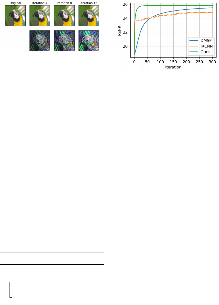
Figure 2: Iterative results of our MAP denoiser network (top
row) and the residual w.r.t. the input image (bottom row).
algorithm is as follows: In the first step we optimize
ˆx. For image deblurring this step can be done effi-
ciently in frequency domain using Equation (9). Sec-
ond, we compute ˆz by a single feed-forward step using
our trained MAP denoiser D
∗
. And finally, we update
the variable λ and reiterate until convergence.
We have conducted several experiments on var-
ious datasets to find the best hyper-parameters for
grayscale non-blind image deblurring. We found that
using the DAE standard deviation σ
R
= 7 performs
best in practice. We also found that setting ρ = 1/σ
2
R
,
so that the Equation (5) is balanced, performs best
in practice. Such setting leads to best results on Sun
dataset (Sun et al., 2013), however, the optimal value
for each image might be different. In the experiments
we use 75 iterations of the ADMM algorithm. How-
ever, as shown in Figure 3, 35 iterations is practically
enough for most experiences.
The processing speed and the convergence rate is
very important in all iterative approaches. As shown
in Figure 3, the proposed method converges very
fast compared to DMSP (both methods are solving
the same MAP optimization). A color image from
BSDS300 can be processed using 35 iterations in
about 0.8 seconds on an NVIDIA GTX2080 GPU in-
cluding the data transfer between the host computer
and the device. This makes our method very attractive
and more useful in practice. We also show the conver-
gence speed of IRCNN, where the noise level of the
denoiser is exponentially decayed from 49 to 15. We
note, that the convergence speed of IRCNN may be
significantly increased at the cost of lower PSNR.
Algorithm 1: Optimization steps for non-blind
image deblurring.
input : Degraded image y, blur kernel matrix
K, and noise standard deviation σ
while not converged do
1. ˆx =

K
T
K + σ
2
ρ

−1

K
T
y + σ
2
ρ(ˆz− λ)

2. ˆz = D
∗
( ˆx + λ)
3. λ = λ + ( ˆx − ˆz)
output: MAP estimate output image ˆx.
Figure 3: Convergence speed comparison on an image from
BSDS300. Note that DMSP and the proposed method try to
optimize the same objective. Using the ADMM approach,
we can speed-up the optimization up to 70x faster.
6.3.1 Optimization
To be consistent with other methods, for all the exper-
iments we first blur the ground-truth test image with
the blur kernel. The blurring is done by convolution
with a flipped version of a kernel and only the valid
area is preserved. We also add a Gaussian noise with
the desired standard deviation σ. After the restoration,
we measure the PSNR on the valid area.
Since we optimize ˆx in the frequency domain, the
proposed method works the best when the degrada-
tion is done using circular convolution. However, in
case we receive only the valid area, assuming the cir-
cular convolution leads to high error on the boarders
which gets propagated towards the center in subse-
quent iterations. To alleviate this behaviour and main-
tain the benefit of processing in frequency domain, we
first pad the degraded image by replicating the edges
to the original size. Furthermore, in each iteration, we
first estimate the non-valid area of the y by perform-
ing a cyclic convolution on the current estimate of ˆx
with the kernel. Such treatment leads to plausible re-
sults and yet it is fast enough due to the processing
in the frequency domain. Figure 4 shows the iterative
results of our optimization, where the image is getting
sharper using the proposed denoising prior.
6.3.2 Datasets
We test the method on two different datasets and re-
port the results in Table 2 and Table 3. The first one
is the Sun dataset (Sun et al., 2013) that consists of
80 images with the longest dimension being 924 pix-
els. The dataset contains 8 blur kernels of various
sizes to simulate the degraded images. The second
dataset we use for evaluation is the BSDS300 (Mar-
tin et al., 2001). It consists of 300 images of size
321 × 481, which we convert to gray-scale. We test

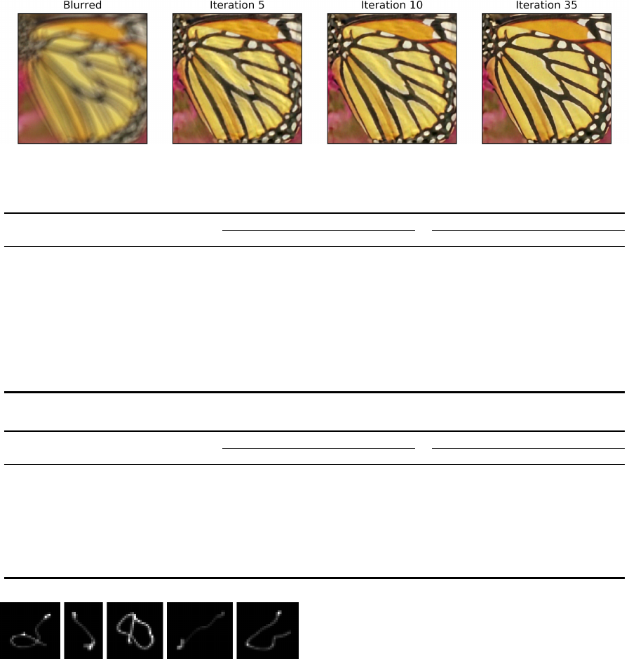
Figure 4: Deblurring results of the ADMMM iterations using the proposed algorithm. Our MAP denoiser network encourages
sharp image edges and removes undesired artifacts.
Table 2: Quantitative comparisons for non-blind image deblurring using two datasets in terms of PSNR.
Sun (Sun et al., 2013) BSDS300 (Martin et al., 2001)
Method σ → 2.55 5.10 7.65 10.2 2.55 5.10 7.65 10.2
FD (Krishnan and Fergus, 2009) 30.79 28.90 27.86 27.14 24.44 23.24 22.64 22.07
EPLL (Zoran and Weiss, 2011) 32.05 29.60 28.25 27.34 25.38 23.53 22.54 21.91
CSF (Schmidt and Roth, 2014) 30.88 28.60 27.65 26.97 24.73 23.60 22.88 22.44
TNRD (Chen and Pock, 2016) 30.03 28.79 28.04 27.54 24.17 23.76 23.27 22.87
DAEP (Bigdeli and Zwicker, 2017) 31.76 29.31 28.01 27.16 25.42 23.67 22.78 22.21
IRCNN (Zhang et al., 2017b) 31.80 30.13 28.93 28.09 25.60 24.24 23.42 22.91
GradNet 7S (Jin et al., 2017) 31.75 29.31 28.04 27.54 25.57 24.23 23.46 22.94
DMSP (Bigdeli et al., 2017) 29.41 29.04 28.56 27.97 25.69 24.45 23.60 22.99
Ours 31.00 29.96 28.96 28.13 26.18 24.52 23.51 22.79
Table 3: Comparison of SSIM scores for non-blind image deblurring using two datasets.
Sun (Sun et al., 2013) BSDS300 (Martin et al., 2001)
Method σ → 2.55 5.10 7.65 10.2 2.55 5.10 7.65 10.2
FD (Krishnan and Fergus, 2009) 0.851 0.787 0.744 0.714 0.664 0.577 0.534 0.492
EPLL (Zoran and Weiss, 2011) 0.880 0.807 0.758 0.721 0.712 0.590 0.521 0.476
CSF (Schmidt and Roth, 2014) 0.853 0.752 0.718 0.681 0.693 0.612 0.558 0.521
TNRD (Chen and Pock, 2016) 0.844 0.790 0.750 0.739 0.690 0.631 0.589 0.550
GradNet 7S (Jin et al., 2017) 0.873 0.798 0.750 0.733 0.731 0.653 0.595 0.552
DMSP (Bigdeli et al., 2017) - - - - 0.740 0.671 0.611 0.563
Ours 0.829 0.817 0.788 0.758 0.768 0.668 0.595 0.540
Figure 5: Blur kernels used in our experiments (Schelten
et al., 2015).
this dataset with the 5 large blur kernels as in (Schel-
ten et al., 2015). These kernels visualized in Figure 5,
have complex structures and lead to challenging de-
blurring tasks.
Figure 6, shows a visual comparison between our
method and several other state-of-the-art techniques.
Our method is able to capture the sharp structures of
the image, while remaining highly efficient compared
to other algorithms.
6.4 Image Inpainting
In addition to the deblurring method, we have also
tested the proposed method on the inpainting prob-
lem. We follow the ADMM approach for image
restoration presented in Section 3. To speed up the
convergence, we initialize our solution ˆx with image
inpainted using a median filter.
6.4.1 Optimization
We conduct the test with 80% of the missing pixels
where we add Gaussian noise with σ = 12 prior to the
remaining pixels. The tested methods are provided
both with the degraded image and with the mask spec-
ifying which pixels were dropped.
In contrast to the image deblurring, we use 300 it-

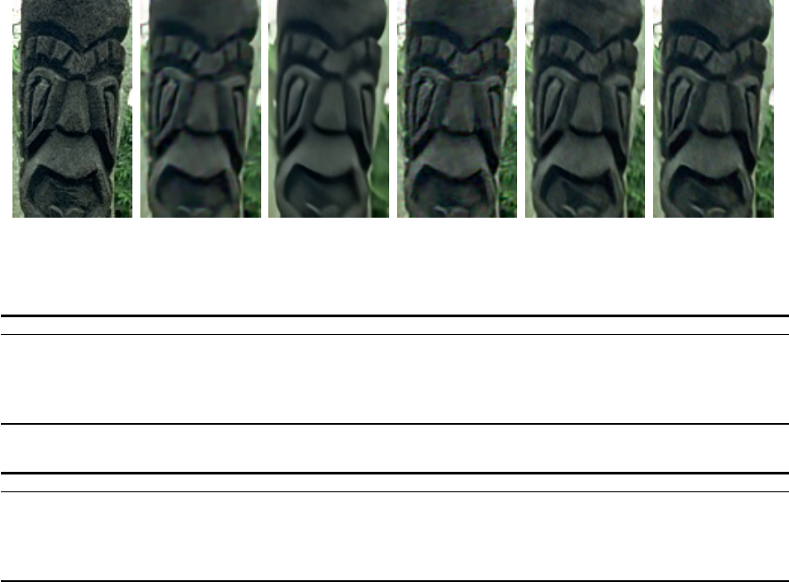
(a) Ground truth (b) EPLL (c) DAEP (d) GradNet 7S (e) DMSP (f) Ours
Figure 6: Visual Comparison of the selected methods for the task of non-blind image deblurring.
Table 4: Inpainting results (PSNR) for 80% of missing pixels and noise with std. deviation of σ = 12.
Method cameraman house peppers Lena Barbara boat hill couple
P&P-BM3D (Venkatakrishnan et al., 2013) 24.43 30.78 26.56 29.47 24.12 26.53 27.44 26.71
IRCNN (Zhang et al., 2017b) 24.59 30.19 26.94 29.52 25.49 26.58 27.55 26.62
IDBP-BM3D (Tirer and Giryes, 2018) 24.51 31.14 26.79 29.69 25.06 26.64 27.61 26.77
IDBP-CNN (Tirer and Giryes, 2018) 24.14 30.92 27.17 29.80 23.61 26.78 27.70 26.80
Ours 23.17 30.32 26.01 29.44 24.30 26.81 28.40 26.77
Table 5: Inpainting results (SSIM) for 80% of missing pixels and noise with std. deviation of σ = 12.
Method cameraman house peppers Lena Barbara boat hill couple
P&P-BM3D (Venkatakrishnan et al., 2013) 0.774 0.839 0.807 0.818 0.705 0.707 0.683 0.734
IRCNN (Zhang et al., 2017b) 0.781 0.835 0.813 0.820 0.758 0.723 0.706 0.736
IDBP-BM3D (Tirer and Giryes, 2018) 0.775 0.844 0.816 0.824 0.738 0.712 0.691 0.738
IDBP-CNN (Tirer and Giryes, 2018) 0.786 0.843 0.830 0.836 0.731 0.738 0.714 0.752
Ours 0.757 0.808 0.814 0.803 0.741 0.721 0.707 0.735
erations of the ADMM algorithm. Moreover, in each
iteration, we use 200 steps of gradient descent opti-
mization to approximate Equation (5) of the ADMM.
6.4.2 Dataset
We evaluate the methods using PSNR and SSIM
scores on classical dataset consisting of images of
cameraman, house, peppers, Lena, Barbara, boat,
hill, and couple.
Tables 4, 5 show the PSNR and SSIM scores of
our method compared to the state-of-the-art. Again,
our method can achieve state-of-the-art results for the
task of image inpainting. Note that we use the same
MAP denoising network as in the previous experi-
ments. We also visualize qualitative results in Fig-
ure 7, where our method can successfully recover
80% of the missing pixels from the input image.
7 CONCLUSIONS
We discussed the challenges of using the plug-and-
play denoising in ADMM optimization for MAP es-
timation. We presented an approach for learning an
end-to-end neural network to perform MAP denois-
ing. We used this network in an ADMM framework
to perform generic image restoration tasks. Our theo-
retical results show that we can guarantee to minimize
the MAP objective using the proposed training strat-
egy. And our experimental validation showed that our
method has significant improvement in speeding up
the MAP optimization, compared to other explicit ap-
proaches. Over all, other method supports the theoret-
ical guarantees of MAP estimation, and at the same
time benefits from the fast performance of other ap-
proaches without such guarantee.
ACKNOWLEDGEMENTS
Financial support from the CSEM Data Program is
grateully acknowledged. Authors would also like to
thank Laura Bujouves for her insightful comments.

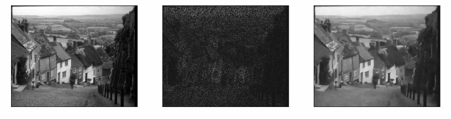
Figure 7: Image inpainting example. Left: Original image, Middle: Degraded image with 80% of the pixels set to zero,
Right: Inpainted image using our method.
REFERENCES
Ahmad, R., Bouman, C. A., Buzzard, G. T., Chan, S.,
Reehorst, E. T., and Schniter, P. (2019). Plug and
play methods for magnetic resonance imaging. arXiv
preprint arXiv:1903.08616.
Bigdeli, S. A. and Zwicker, M. (2017). Image restora-
tion using autoencoding priors. arXiv preprint
arXiv:1703.09964.
Bigdeli, S. A., Zwicker, M., Favaro, P., and Jin, M. (2017).
Deep mean-shift priors for image restoration. In
Advances in Neural Information Processing Systems,
pages 763–772.
Chang, J.-H. R., Li, C.-L., Poczos, B., Kumar, B. V., and
Sankaranarayanan, A. C. (2017). One network to
solve them all-solving linear inverse problems using
deep projection models. In ICCV, pages 5889–5898.
Chen, Y. and Pock, T. (2016). Trainable nonlinear reaction
diffusion: A flexible framework for fast and effective
image restoration. IEEE transactions on pattern anal-
ysis and machine intelligence, 39(6):1256–1272.
Heide, F., Steinberger, M., Tsai, Y.-T., Rouf, M., Paj ˛ak, D.,
Reddy, D., Gallo, O., Liu, J., Heidrich, W., Egiazar-
ian, K., et al. (2014). Flexisp: A flexible camera image
processing framework. ACM Transactions on Graph-
ics (TOG), 33(6):231.
Isola, P., Zhu, J.-Y., Zhou, T., and Efros, A. A. (2017).
Image-to-image translation with conditional adversar-
ial networks. In Proceedings of the IEEE conference
on computer vision and pattern recognition, pages
1125–1134.
Jin, M., Roth, S., and Favaro, P. (2017). Noise-blind image
deblurring. In Proceedings of the IEEE Conference
on Computer Vision and Pattern Recognition, pages
3510–3518.
Krishnan, D. and Fergus, R. (2009). Fast image deconvo-
lution using hyper-laplacian priors. In Advances in
neural information processing systems, pages 1033–
1041.
Martin, D., Fowlkes, C., Tal, D., and Malik, J. (2001).
A database of human segmented natural images and
its application to evaluating segmentation algorithms
and measuring ecological statistics. In Proc. 8th Int’l
Conf. Computer Vision, volume 2, pages 416–423.
Reehorst, E. T. and Schniter, P. (2018). Regulariza-
tion by denoising: Clarifications and new interpreta-
tions. IEEE Transactions on Computational Imaging,
5(1):52–67.
Schelten, K., Nowozin, S., Jancsary, J., Rother, C., and
Roth, S. (2015). Interleaved regression tree field cas-
cades for blind image deconvolution. In 2015 IEEE
Winter Conference on Applications of Computer Vi-
sion, pages 494–501. IEEE.
Schmidt, U. and Roth, S. (2014). Shrinkage fields for ef-
fective image restoration. In Proceedings of the IEEE
Conference on Computer Vision and Pattern Recogni-
tion, pages 2774–2781.
Sønderby, C. K., Caballero, J., Theis, L., Shi, W., and
Huszár, F. (2016). Amortised map inference for image
super-resolution. arXiv preprint arXiv:1610.04490.
Sun, L., Cho, S., Wang, J., and Hays, J. (2013). Edge-based
blur kernel estimation using patch priors. In IEEE In-
ternational Conference on Computational Photogra-
phy (ICCP), pages 1–8. IEEE.
Tirer, T. and Giryes, R. (2018). Image restoration by itera-
tive denoising and backward projections. IEEE Trans-
actions on Image Processing, 28(3):1220–1234.
Ulyanov, D., Vedaldi, A., and Lempitsky, V. (2018). Deep
image prior. In Proceedings of the IEEE Conference
on Computer Vision and Pattern Recognition, pages
9446–9454.
Venkatakrishnan, S. V., Bouman, C. A., and Wohlberg, B.
(2013). Plug-and-play priors for model based recon-
struction. In 2013 IEEE Global Conference on Signal
and Information Processing, pages 945–948. IEEE.
Zhang, C., Bengio, S., Hardt, M., Recht, B., and Vinyals, O.
(2016). Understanding deep learning requires rethink-
ing generalization. arXiv preprint arXiv:1611.03530.
Zhang, K., Zuo, W., Chen, Y., Meng, D., and Zhang, L.
(2017a). Beyond a gaussian denoiser: Residual learn-
ing of deep cnn for image denoising. IEEE Transac-
tions on Image Processing, 26(7):3142–3155.
Zhang, K., Zuo, W., Gu, S., and Zhang, L. (2017b). Learn-
ing deep cnn denoiser prior for image restoration. In
Proceedings of the IEEE conference on computer vi-
sion and pattern recognition, pages 3929–3938.
Zoran, D. and Weiss, Y. (2011). From learning models of
natural image patches to whole image restoration. In
2011 International Conference on Computer Vision,
pages 479–486. IEEE.