Inferring Low-level Mental States of Mobile Users from Plethysmogram

Features by Regression Models based on Kernel Method

Toshiki Iso

Research Laboratories, NTT DOCOMO, INC., Kanagawa, Japan

Keywords:

Earlobe Plethysmogram, Low-level Mental States, Gaussian Process Regression, Support Vector Regression,

Feature Extraction, Automatic Relevance Determination, LF/HF, Lyapunov Coefﬁcient.

Abstract:

To infer user’s response when using mobile services without direct interrogation, we propose an algorithm

that analyzes earlobe plethysmograms to determine low-level mental states such as ‘relax’, ‘concentration’,

‘awake’. We use subject’s responses acquired in a subjective evaluation as indicative of low-level mental

states when subjects use some mobile contents. In order to draw an inference of low-level mental states based

on plethysmogram features, our proposed algorithm uses a kernel-based regression model such as Gaussian

Process Regression (GPR) or Support Vector Regression (SVR). Our evaluations show that features effective

for inferring user’s low-level mental states can be extracted from plethysmograms by using regression and

Automatic Relevance Determination (ARD); the regression performance of GPR and SVR are described.

1 INTRODUCTION

Service providers want to be able to detect the

user’s low-level mental states such as ‘concentra-

tion’ and ‘vagueness’. Because plethysmogram can

be easily detected by non-invasive means (Allen,

2007), low-level mental states based on plethysmo-

gram are being used for medical applications such

as the diagnosis of dementia in aged people(Oyama-

Higa et al., 2006), analysis of physio-psychological

status(Oyama-Higa and Miao, 2005), and detecting

snooze driving(Vicente et al., 2016).Recently, Inter-

net service providers also want to know the user’s

low-level mental states in order to discover their re-

sponses for improving the services. In more detail,

the desired user responses are not high-level mental

states such as positive or negative feelings about the

content, but whether the services enhance or weaken

the user’s interest. Information on whether the user

is actively searching for desired contents or aimlessly

accessing web pages allows the service provider to

control the type of banner advertisements displayed.

While plethysmography appears attractive in esti-

mating the user’s low-level mental states, there is no

commonly accepted method for detecting the states

with minimal user interference. Diagnosis of ap-

nea syndrome(Loube et al., 1999),(Romem et al.,

2014) and mental illness and detecting drunk driv-

ing(Murata et al., 2011) process plethysmograms

gathered by attaching sensors to the subject’s body.

Fixing a sensor to the user’s ﬁnger makes mobile ser-

vices very cumbersome and unattractive. We need

a method with minimal user constraints that allows

context-aware services to realize effective control

of advertisements depending on the user’s low-level

mental states. Service providers currently are con-

ducting questionnaires to determine the user’s re-

sponses. While overall service impressions can be

gathered, details are difﬁcult to acquire because users

have difﬁculty remembering and verbalizing their im-

pressions. One method detects the user’s responses

by analyzing Internet access history, but it is impos-

sible to distinguish between focused and non-focused

browsing. Another proposed method analyzes user

eye movements(Wong et al., 2014). Unfortunately,

combining eye-tracking with smartphone device use

in mobile environments is not realistic.

Y. Cho et al. proposed to infer mental stress from

photoplethysmographic data acquired from RGB and

thermal images(Cho et al., 2019),(Alafeef, 2017)This

scheme is difﬁcult to use in mobile environments be-

cause of its constraints such as assuming the user’s

ﬁnger and face occupy ﬁxed positions. More impor-

tantly, as photoplethysmography extracts only heart

rate features, it can detect few mental states. How-

ever, if plethysmograms can be detected without un-

due user constraints, it would be useful for inferenc-

ing low-level mental states because apnea syndrome,

250

Iso, T.

Inferring Low-level Mental States of Mobile Users from Plethysmogram Features by Regression Models based on Kernel Method.

DOI: 10.5220/0008977002500257

In Proceedings of the 13th International Joint Conference on Biomedical Engineering Systems and Technologies (BIOSTEC 2020) - Volume 4: BIOSIGNALS, pages 250-257

ISBN: 978-989-758-398-8; ISSN: 2184-4305

Figure 1: Wearable device mounted on earlobe for plethys-

mogram capture.

mental illness, and detecting snooze driving, use fea-

tures extracted from plethysmogram data such as

LF/HF and Lyapunov by chaos analysis(Oyama-Higa

and Miao, 2005),(Sumida et al., 2000). Low-level

mental states can be detected by analyzing plethysmo-

grams as heart rate control is strongly inﬂuenced by

sympathetic nerves. Though plethysmograms are be-

ing used for the analysis of low-level mental states, it

is not clear how to extract valid features from plethys-

mograms nor which statistical analysis models are

valid for recognizing the mental states.

In order to infer low-level mental states, we pro-

pose a method that uses earlobe plethysmograms;

it uses the already proposed wearable mobile de-

vice that places no undue constraints on user opera-

tions(Kimura et al., 2013). The interface sets plethys-

mogram sensors on the ear lobes areas of the user.

We identify which plethysmogram features are valid

for recognizing the key mental states and evaluate the

performance of different statistical analysis models in

inferring low-level mental states.

In the next section, we describe feature extrac-

tion from plethysmograms and subjective evalua-

tion features for determining low-level mental states.

We then explain our proposals for selecting plethys-

mogram features, regression analysis of plethysmo-

grams, and deriving subjective evaluation features by

kernel-based regression techniques. Finally, we ex-

plain our experiments on inferencing low-level men-

tal states and future work.

2 FEATURE EXTRACTION

In this section, we describe feature extraction from

plethysmograms and the subjective evaluation fea-

tures needed for determining low-level mental states.

2.1 Subjective Evaluation Features of

Low-level Mental States

In order to determine low-level mental states, 13 sub-

jects wearing earlobe plethysmogram sensors were

subjectively evaluated; they accessed eight types of

mobile services (each for about 5 to 15 minutes) on

a smartphone: The contents contained the subject’s

favorite contents such as movies and games and con-

tents uncomfortable on a biological level such lis-

tening to strange noise. These contents were in-

tended to force the subjects to experience known low-

level mental states. Immediately after the experi-

ments, videos of the services experienced were re-

viewed. The 13 subjects scored each subjective eval-

uation items (eight types) with one of seven numeri-

cal levels (seven degrees) every 5 minutes. The eight

subjective evaluation items were ‘boredom’, ‘concen-

tration’, ‘satisfaction’, ‘interest’, ‘joy’, ‘enjoyment’,

‘anger’, and ‘sadness’; this was done because it is eas-

ier for subjects to indicate their feelings about service

contents than their low-level mental states such as ‘re-

lax’ and ‘concentration’. However, in order to obtain

reliable evaluation data, only scores that the subject

felt conﬁdent in making were used. Figure 2 plots

the relationships between the scores of the subjective

evaluation items as indicated by a subject’s watch-

ing a favorite video. We can see that these relation-

ships have little direct correspondance other than the

relationship between “satisfaction” and ‘interest’. In

other words, the subjective evaluation items are ba-

sically independent of each other. Then, under the

assumption that all scores of the subjective evaluation

items are indicative of low-level mental states such as

‘relax’ and ‘concentration’, we deﬁne low-level men-

tal state y(t) at time t as follows:

y(t) =

(Sr ∗ M)

∑

k=1

Score

(t) (1)

where Score

(t) represents the score of the kth evalu-

ation item at time t by the subject. Sr and M represent

number of judgements possible (seven degrees) and

number of subjective evaluation items (eight types),

respectively. Using just the direct summation of the

subjective evaluation scores, not the items individu-

ally, fails to distinguish positive from negative low-

level mental states. Note that y(t) does offers ser-

vice providers valuable information about the user’s

responses.

2.2 Plethysmogram Feature

As described above, we obtained earlobe plethysmo-

grams of 13 subjects when using mobile services. In

Inferring Low-level Mental States of Mobile Users from Plethysmogram Features by Regression Models based on Kernel Method

251

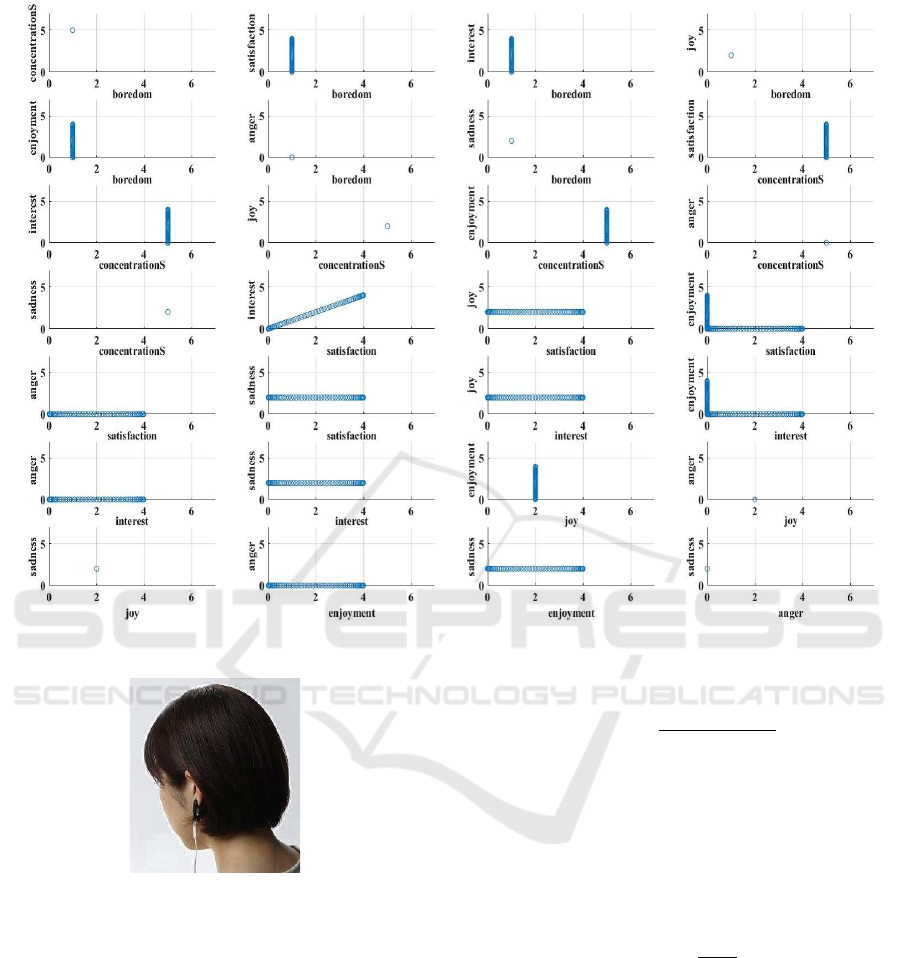
Figure 2: Linearity relations between subjective evaluation items.

Figure 3: The earlobe plethysmogram device made by

TAOS Institute, Inc.

the experiments, we used the earlobe plethysmogram

device made by TAOS Institute, Inc. (see Figure 3)

because more accurate data can be extracted by tight

coupling to the subject’s earlobe.

The upper part of Figure 4 shows typical time-

series data from the earlobe plethysmogram device.

We extract four features from the data.

Feature Type1: Second Derivative

The upper part of Figure 4 plots the second deriva-

tive of the plethysmogram(Mohamed, 2012). By de-

tecting ﬁve extreme values such as from a-wave to

e-wave, we calculate SDPTGAI (second derivative of

plethysmogram aging index) at time t as follows:

(t) =

(b − c − d − e)

(2)

The SDPTGAI feature represents a measure of

vascular stiffness.

Feature Type2: Heart Rate Variability

(t) at time t can be calculated as peak-to-peak inter-

val times; that is, the second derivative of plethysmo-

gram. Thus heart rate x

(t) at time t can be calculated

from PPI x

(t) as follows:

(t) =

(t)

(3)

Feature Type3: Frequency Spectrum

After removing outliers from PPI x

(t), we calculate

the power spectral density PSD

all

(t) from t − ws

f s

to t + ws

f s

/2 where window size is set at 30[sec]. We

then extract the low-frequency component PSD

(t)

in the frequency range from 0.04[Hz] to 0.15[Hz]

and the high-frequency component PSD

HF(t)

in the

frequency range from 0.15[Hz] to 0.40[Hz] from

PSD

all

(see Figure 5).The low-frequency component

represents the responses of blood pressure ﬂuctua-

tion (Mayer wave) and sympathetic activity(Shaffer

BIOSIGNALS 2020 - 13th International Conference on Bio-inspired Systems and Signal Processing

252

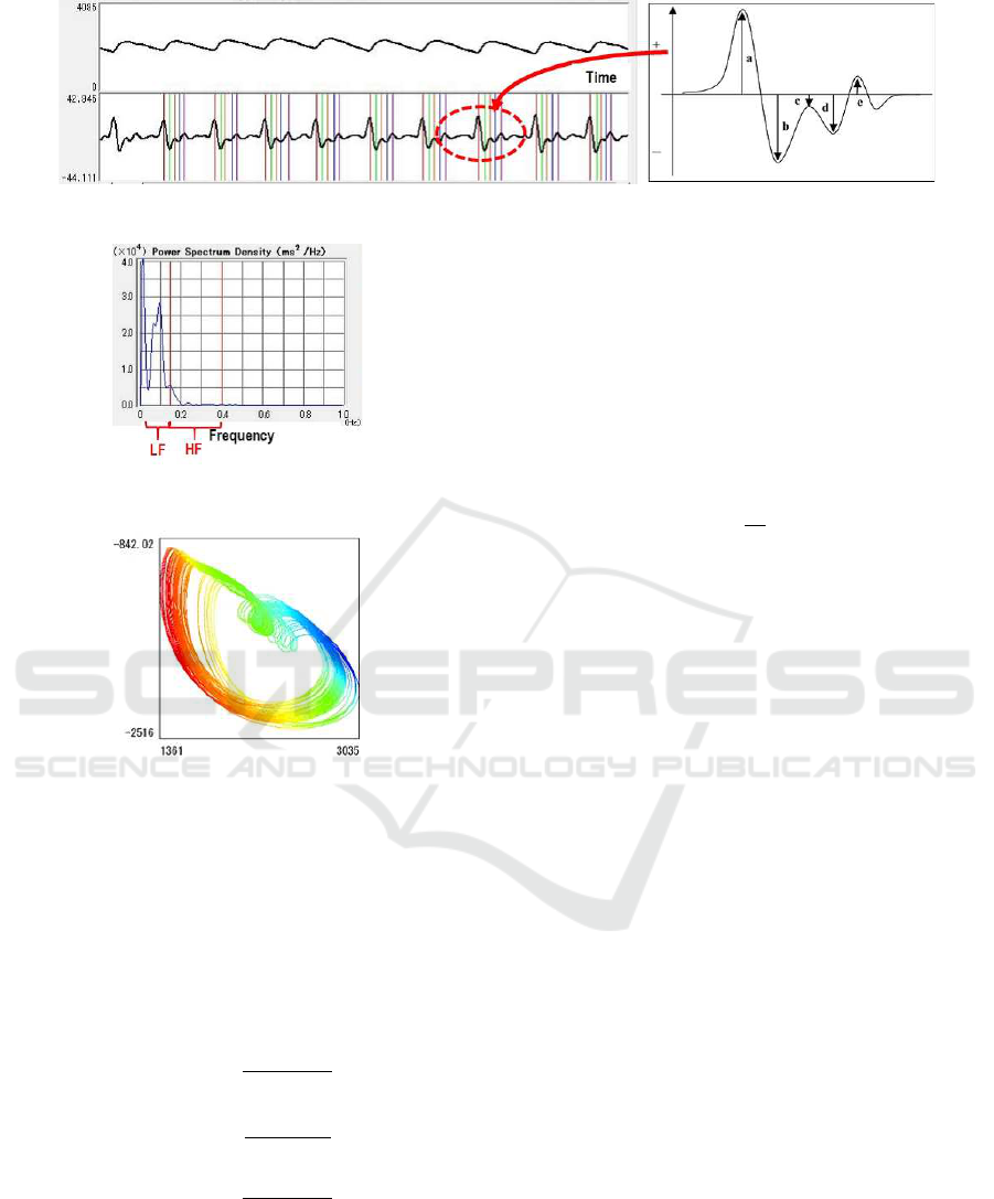
Figure 4: Plethysmogram and second derivative of plethysmogram.

Figure 5: Low-frequency component and high-frequency

component.

Figure 6: Chaos attractor based on plethysmogram (trajec-

tory projected).

and Ginsberg, 2017). The high-frequency compo-

nent represents parasympathetic activity and respira-

tory variation. While the high-frequency component

is present only when the parasympathetic nerve is

tense (autonomic nerve is quiescent as in ‘relax’), the

low-frequency component is present when both the

parasympathetic and sympathetic nerve are tense. We

deﬁne Feature Type3 as follows:

(t) = log

PSD

(t)

PSD

all

(t)

(4)

(t) = log

PSD

(t)

PSD

all

(t)

(5)

(t) = log

PSD

(t)

PSD

(t)

(6)

MeanHR x

(t) is calculated as the mean heart rate

from t − ws

f s

/2 to t + ws

f s

/2.

Feature Type4: Chaos Attractor

According to Tsuda et al. (Tsuda et al., 1992),

plethysmograms can be represented as a function of

four dimensional state variables, while the trajectory

mirrors a four dimensional chaos attractor. Figure 6

shows a typical trajectory of a four-dimensional chaos

attractor projected into two dimensions. Based on

Sano and Sawada(Sano and Sawada, 1985), we cal-

culate the Lyapunov exponent from the four dimen-

sional chaos attractor as follows:

(t) = max

d=1,2,3,4

(7)

where window size is set at 17.5[sec]. Then,

= lim

n→∞

nτ

∑

j=1

lnA

(8)

where d is chaos attractor dimension, n is the num-

ber of sampled data points on the attractor, A

is a

linear operator matrix of trajectory tangent vectors,

τ is the evolution of time interval, and e

is a basis

vector of the tangent space. If λ is positive, the tra-

jectory demonstrates chaotic behavior, but, if λ is not

positive, it is characteristic of the turbulence of chaos,

which has the potential to be a criterion for distin-

guishing low-level mental states. We calculate the en-

tropy of the chaos attractor x

(t) as follows:

(t) = −

∑

i=1

log p

(9)

where p

represents the percentage of all sampled

points on the chaos attractor that go through the ith

small area in phase space, and N is the number of

small areas in phase space. As the entropy represents

chaos turbulence, it also has the potential to be a valid

criterion for low-level mental states. Feature Type1 to

Feature Type4 are deﬁned at time t. In particular, be-

cause Feature Type3 and Type4 are calculated using

time windows, they can contain some characteristics

evidenced in the periods around time t. The above

nine feature are different from one another in terms of

time sampling. Then, after normalizing each feature

against maximum and minimum values, they are syn-

chronized by using time interpolation using the time

resolution (sampling frequency 100[Hz]) of

X = (x

(t),x

(t),··· ,x

(t))

(10)

To preprocess the time series data, we use the

time difference of X . This is necessary because X is

Inferring Low-level Mental States of Mobile Users from Plethysmogram Features by Regression Models based on Kernel Method

253

Figure 7: Time-Stationarity of feature vector based on time difference data and raw data.

likely to contain sensor noise and daily ﬂuctuations

such as the effects of ‘human feelings’.

Time-Stationarity of Feature Vector

In order to extract more stable data for regression

analysis, we calculate mean and standard deviation in

local time for the above raw data and time difference

data as basic descriptive statistical values. Figure 7

shows the results gained from each mobile service.

We can conﬁrm that the time difference data exhibits

more time-stationarity than the raw data. Hereafter,

the time differences on X are used as input data for

inferencing low-level mental states.

3 INFERENCING LOW-LEVEL

MENTAL STATES

3.1 Regression Models

Recently, deep learning methods have been applied

in a variety of applications, but they need large

amounts of high quality training data, which are very

difﬁcult to collect. Therefore, we need a regres-

sion method that can construct mapping feature vec-

tors from plethysmogram data without over-ﬁtting.

To avoid over-ﬁtting in constructing the regression

model, we focus on kernel-function-based approaches

with constraints. This is because it offers ﬂexible

regression with kernel function and suppresses over-

ﬁtting.

3.1.1 Gaussian Process Regression

We outline below the Gaussian Process Regression

(GPR)(Rasmussen and Williams, 2006). When joint

probability p(y

,··· ,y

) of output data points y

(i =

1,2,··· ,N) corresponding to N-number of input data

vectors X

= (x

,··· ,x

)

follows a multivariate

Gaussian distribution; that is, the weight matrix w sat-

isﬁes

w ∼ N (0,λ

I) (11)

the estimated output data

y(= ( ˆy

,··· , ˆy

)) is given

as follows:

y ∼ N (0,λ

ΦΦ

) (12)

where λ

and Φ are variance of w and a matrix of basis

functions, respectively. K = λ

ΦΦ

is a covariance

matrix of λΦ(X

). Choosing a kernel function that

ensures K is a positive deﬁnite matrix, yields the es-

timated output data

y. GPR uses Bayesian estimation

based on a kernel function, it avoids the over-ﬁtting

problem. GPR is used for not only regression but

also Bayesian optimization for determining the opti-

mal parameters in deep learning and feature selection

as described below. We can analyze the ﬂuctuations

of output data

y to identify low-level mental states

because standard deviations of Gaussian distributions

can represent ﬂuctuations in regression as GPR can

basically inference the Gaussian distribution at each

point of

3.1.2 Support Vector Regression

We outline Support Vector Regression (SVR)(Smola

and Sch

olkopf, 2004). Unlike SVM (Support Vector

BIOSIGNALS 2020 - 13th International Conference on Bio-inspired Systems and Signal Processing

254

Machine), SVR uses criterion function S

, which min-

imizes error function h between the estimated output

data

y and the actual output data y (not the number of

misclassiﬁed data), as follows:

kwk

∑

d=1

y − y) (13)

where D represents the dimension of y.

This also avoids over-ﬁtting because SVR also

uses constraint condition

kwk

. Therefore, SVR

can yield sparse regression because it applies L1-

optimization to criterion function S

. Note that, GPR

is a generative model approach based on Ridge re-

gression with a kernel trick, and so is more sensitive

to data than SVR.

3.2 Selection of Plethysmogram Feature

As described in the Introduction, different applica-

tions use different plethysmogram features. We iden-

tify the valid plethysmogram features by Automatic

Relevant Determination (ARD) with GPR(Wipf and

Nagarajan, 2008). ARD can estimate the degree

of contribution of explanatory variables to objective

variables. In the above section, when we use GPR,

we need to select the kernel function. For the purpose

of feature selection, we use the squared exponent ker-

nel function as follows:

K(x

) = exp(−

∑

d=1

(

− x

)) (14)

where x

and x

are explanatory variables vectors of

the n-th and n

-th data, respectively. x

represents

the d-th explanatory variable vectors of the n-th data.

and D represent characteristic length scale asso-

ciated with d-th component in explanatory variables

and dimension of explanatory variables vectors, re-

spectively. Increasing the characteristic length scale,

, decreases the contribution of the d-th component

in the explanatory variables. Therefore, we analyze

which features extracted from plethysmograms are

valid for inferencing low-level mental states.

4 EXPERIMENTAL RESULTS

We use GPR and SVR to make two regression mod-

els. Both use a Gaussian kernel as the kernel function.

The regression deals with analog values of y as low-

level mental states. Our regression evaluations em-

ploy k-fold cross validation(k = 5). We combine the

data from all subjects because some subjects exhib-

ited many responses in their evaluation scores, while

other subjects demonstrate scant responses.

4.1 Regression with GPR and SVR

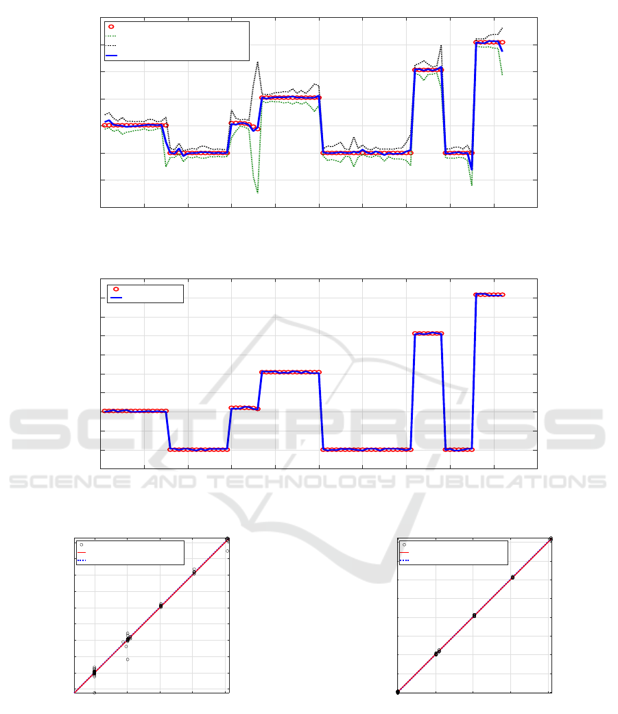
Figures 8 and Figures 9 show the regression results

yielded by GPR and SVR, respectively. Figures 10

and Figures 11 plot the regression coefﬁcients for

GPR and SVR, respectively. For GPR we show

the conﬁdence intervals based on standard deviation.

Both regression models have only small differences

between real and estimated values. As their regres-

sion coefﬁcients are about 0.98, both methods are

valid for inferencing low-level mental states. They

use the kernel function based approach and their cri-

terion contains a constraint for avoiding over-ﬁtting.

As the data set used did not have ﬁne variations, SVR

as a sparse regression is better than GPR. But, GPR

can provide conﬁdence scores for regression at each

data point because of its Bayesian approach. The con-

ﬁdence scores are useful for real applications. As it is

basically difﬁcult to collect subjective evaluation data

in real services, deep learning models are not suitable

as they need big data sets of subjective evaluations to

create adequate training for accurate parameter deter-

mination. The standard deviations of each point in

yielded by GPR represent estimation variance. There-

fore, to realize more accurate regression, we should

use criteria that select high-quality data sets that yield

strong correspondence between input data (plethys-

mogram feature) and output data (subjective evalua-

tion).Data sets that contain big ﬂuctuations in features

extracted from plethysmograms or subjective evalua-

tions will negatively inﬂuence the regression analyses

by either GPR or SVR.

4.2 Feature Selection for Inferencing

Low-level Mental States

Figure 12 shows feature selection by using ARD with

GPR. It shows that Feature Type3 (frequency spec-

trum) and Type4 (chaos attractor) yield valid infer-

encing of low-level mental states. We consider that

these features are difﬁcult to extract with accuracy

because Feature Type1 (second derivative of plethys-

mogram) and Type2 (heart rate variability) use infor-

mation of second derivative of plethysmogram and so

suffer from numerical error in detecting local maxi-

mum or minimum and calculating the derivative. In

particular, Feature Type1 is not valid as each person

has a different level of vascular ﬂexibility. On the

other hand, Feature Type3 (frequency spectrum) and

Type4 offer stable feature extraction as they offer rich

information in time windows.

Inferring Low-level Mental States of Mobile Users from Plethysmogram Features by Regression Models based on Kernel Method

255

0 10 20 30 40 50 60 70 80 90 100

Input Data (Feature Vector of Plethysmogram)

-0.04

-0.02

0.02

0.04

0.06

0.08

0.1

Output Data (Subjective Evaluation)

Comparison Of Validation Data and Estimated Data (GPR)

Validation Data

Low Confidence Interval (95%)

High Confidence Interval (95%)

Estimated Data

Figure 8: Regression by GPR.

0 10 20 30 40 50 60 70 80 90 100

Input Data (Feature Vector of Plethysmogram)

-0.01

0.01

0.02

0.03

0.04

0.05

0.06

0.07

0.08

0.09

Output Data (Subjective Evaluation)

Comparison Of Validation Data and Estimated Data (SVR)

Validation Data

Estimated Data

Figure 9: Regression by SVR.

0 0.02 0.04 0.06 0.08

Validation Data

-0.01

0.01

0.02

0.03

0.04

0.05

0.06

0.07

0.08

Estimated Data ~= 1*Validation Data + -0.00017

Regression Evaluation (GPR) : R=0.99642

Validation Data

Fitting Line

Estimated data = Validation Data

Figure 10: Evaluation of Regression by GPR.

5 CONCLUSION

Our experimental evaluation showed that both GPR

and SVR offer good regression analyses of plethys-

mogram features and subjective evaluations; accord-

ing to cross validation, the regression coefﬁcients are

0 0.02 0.04 0.06 0.08

Validation Data

0.01

0.02

0.03

0.04

0.05

0.06

0.07

0.08

Output ~= 1*Validation Data + 8.5e-05

Regression Evaluation (SVR) : R=0.99989

Validation Data

Fitting Line

Estimated Data = Validation Data

Figure 11: Evaluation of Regression by SVR.

about 0.98. As a result, we reveal the potential to

detect low-level mental states by Earlobe Plethysmo-

gram sensors mounted on wearable devices. More-

over, feature selection by ARD with GPR showed

that Feature Type3 (frequency spectrum) and Type4

(chaos attractor) offer valid inferencing of low-level

mental states. In future work, we will improve regres-

BIOSIGNALS 2020 - 13th International Conference on Bio-inspired Systems and Signal Processing

256

Relevance Of Each Features of Plethysmogram

SDPTGAI

heartRate

RRInterval

logHF

logLF

logLFPHF

MeanHR

Lyapunov

entropy

Feature of Plethysmogram

-1.4

-1.2

-1

-0.8

-0.6

-0.4

-0.2

0.2

0.4

Log of length scale

Figure 12: Feature Selection by using ARD with the GPR.

sion accuracy by selecting good quality data sets

based on standard deviation from GPR or ﬁnding

other criteria for discriminating low-level mental

states.

ACKNOWLEDGEMENTS

The author would like to thank Mr. Gesshi Higashida,

TAOS Institute, Inc. R & D Department for his tech-

nical support in the experiments.

REFERENCES

Alafeef, M. (2017). Smartphone-based photoplethysmo-

graphic imaging for heart rate monitoring. Journal of

Medical Engineering & Technology, 41(5):387–395.

PMID: 28300460.

Allen, J. (2007). Photoplethysmography and it application

in clinical physiological measurement. Physiological

measurement, 28:R1–39.

Cho, Y., Julier, S. J., and Bianchi-Berthouze, N. (2019).

Instant stress: Detection of perceived mental stress

through smartphone photoplethysmography and ther-

mal imaging. JMIR Ment Health, 6(4):e10140.

Kimura, S., Fukuomoto, M., and Horikoshi, T. (2013).

Eyeglass-based hands-free videophone. Proceedings

of the 2013 International Symposium on Wearable

Computers, pages 117–124.

Loube, D. I., Andrada, T., and Howard, R. S. (1999). Accu-

racy of respiratory inductive plethysmography for the

diagnosis of upper airway resistance syndrome. Chest,

115(5):1333 – 1337.

Mohamed, E. (2012). On the analysis of ﬁngertip photo-

plethysmogram signals. Current cardiology reviews

vol. 8,1 14-25.

Murata, K., Fujita, E., Kojima, S., Maeda, S., Ogura, Y.,

Kamei, T., Tsuji, T., Kaneko, S., Yoshizumi, M., and

Suzuki, N. (2011). Noninvasive biological sensor sys-

tem for detection of drunk driving. IEEE Transactions

on Information Technology in Biomedicine, 15(1):19–

25.

Oyama-Higa, M. and Miao, T. (2005). Representation

of a physio-psychological index through constellation

graphs. In ICNC (1)’05, pages 811–817.

Oyama-Higa, M., Miao, T., and Mizuno-Matsumoto, Y.

(2006). Analysis of dementia in aged subjects through

chaos analysis of ﬁngertip pulse waves. In 2006 IEEE

International Conference on Systems, Man and Cy-

bernetics, volume 4, pages 2863–2867.

Rasmussen, B. C. E. and Williams, C. K. I. (2006). Gaus-

sian Processes for Machine Learning . The MIT Press.

Romem, A., Romem, A., Koldobskiy, D., and Schar

(2014). Diagnosis of obstructive sleep apnea using

pulse oximeter derived photoplethysmographic sig-

nals. Journal of Clinical Sleep Medicine, 10(3):285–

290.

Sano, M. and Sawada, Y. (1985). Measurement of the lya-

punov spectrum from a chaotic time series. Phys. Rev.

Lett., 55:1082–1085.

Shaffer, F. and Ginsberg, J. P. (2017). An overview of heart

rate variability metrics and norms. Frontiers in Public

Health, 5:258.

Smola, A. J. and Sch

olkopf, B. (2004). A tutorial on

support vector regression. Statistics and Computing,

14(3):199–222.

Sumida, T., Arimitu, Y., Tahara, T., and Iwanaga, H. (2000).

Mental conditions reﬂected by the chaos of pulsation

in capillary vessels. International Journal of Bifurca-

tion and Chaos, 10(09):2245–2255.

Tsuda, I., Tahara, T., and Iwanaga, H. (1992). Chaotic pul-

sation in human capillary vessels and its dependence

on mental and physical conditions. International Jour-

nal of Bifurcation and Chaos, 02(02):313–324.

Vicente, J., Laguna, P., Bartra, A., and Bail

on, R. (2016).

Drowsiness detection using heart rate variability.

Medical & Biological Engineering & Computing,

54(6):927–937.

Wipf, D. P. and Nagarajan, S. S. (2008). A new view of au-

tomatic relevance determination. In Platt, J. C., Koller,

D., Singer, Y., and Roweis, S. T., editors, Advances

in Neural Information Processing Systems 20, pages

1625–1632. Curran Associates, Inc.

Wong, W., Bartels, M., and Chrobot, N. (2014). Practi-

cal eye tracking of the ecommerce website user ex-

perience. In Stephanidis, C. and Antona, M., edi-

tors, Universal Access in Human-Computer Interac-

tion. Design for All and Accessibility Practice, pages

109–118, Cham. Springer International Publishing.

Inferring Low-level Mental States of Mobile Users from Plethysmogram Features by Regression Models based on Kernel Method

257