
Self-supervised Depth Estimation
based on Feature Sharing and Consistency Constraints
Julio Mendoza
a
and Helio Pedrini
b
Institute of Computing, University of Campinas, Campinas-SP, 13083-852, Brazil
Keywords:
Depth Estimation, Self-supervised Learning, Multi-task Learning, Consistency Constraints.
Abstract:
In this work, we propose a self-supervised approach to depth estimation. Our method uses depth consistency to
generate soft visibility mask that reduces the error contribution of inconsistent regions produced by occlusions.
In addition, we allow the pose network to take advantage of the depth network representations to produce more
accurate results. The experiments are conducted on the KITTI 2015 dataset. We analyze the effect of each
component in the performance of the model and demonstrate that the consistency constraint and feature sharing
can effectively improve our results. We show that our method is competitive when compared to the state of
the art.
1 INTRODUCTION
Depth and camera motion estimation are key prob-
lems in computer vision that have many applications
such as 3D reconstruction, virtual and augmented
reality, robot navigation, scene interaction, and au-
tonomous driving. Methods proposed for depth and
camera motion estimation relied on exploring the in-
formation of sparse correspondences on various views
of a scene (Triggs et al., 1999; Souza et al., 2018).
However, these methods produce sparse depth maps
and require post-processing to produce dense depth
maps. As well as various problems in computer vi-
sion (Tacon et al., 2019; Santos and Pedrini, 2019;
Concha et al., 2018), deep learning has been suc-
cessfully applied to depth and camera motion estima-
tion. In the supervised deep learning literature, sev-
eral methods have been proposed to learn to regress
both depth and camera motion values in various sce-
narios when ground-truth data is available.
A major drawback of supervised deep learning
methods for depth estimation and camera motion es-
timation is that they require to collect large datasets.
For instance, depth estimation for autonomous driv-
ing is costly because it requires to acquire data with
LIDAR scanners under diverse weather conditions.
Moreover, LIDAR scanners obtain sparse depth maps.
In contrast, unsupervised deep learning methods that
a
https://orcid.org/0000-0001-5820-2615
b
https://orcid.org/0000-0003-0125-630X
do not need ground-truth for depth and camera mo-
tion tasks. Specifically, self-supervised methods that
rely on exploiting geometric relations to reconstruct
frames and use photometric error as learning sig-
nal (Zhou et al., 2017) have been successfully applied.
Moreover, several methods have been proposed to
deal with several aspects of the problem, for instance,
occlusion (Luo et al., 2018), moving objects (Casser
et al., 2019), image resolution (Pillai et al., 2019),
among others.
In this work, we propose a self-supervised method
for depth and camera motion estimation in monocu-
lar videos. Inspired by multi-task learning literature,
where various methods have been proposed that take
advantage of the task similarity and share representa-
tions between tasks, we propose to share the represen-
tations of depth network to camera motion network.
Specifically, we use the feature maps of each layer in
the encoder part of the depth network as input to the
camera motion network by projecting and summing
them to their task-specific feature maps.
Moreover, we investigate a constraint that de-
creases the error contribution of regions with incon-
sistent projected depth values. Thus, the model does
not lose supervision in the early stages of training,
where depth estimates are more prone to have incon-
sistencies.
This text is organized as follows. In Section 2,
we review some relevant methods related to the topic
under investigation. In Section 3, we present the pro-
posed self-supervised depth estimation methodology.
134
Mendoza, J. and Pedrini, H.
Self-supervised Depth Estimation based on Feature Sharing and Consistency Constraints.
DOI: 10.5220/0008975901340141
In Proceedings of the 15th International Joint Conference on Computer Vision, Imaging and Computer Graphics Theory and Applications (VISIGRAPP 2020) - Volume 5: VISAPP, pages
134-141
ISBN: 978-989-758-402-2; ISSN: 2184-4321
Copyright
c
2022 by SCITEPRESS – Science and Technology Publications, Lda. All rights reserved

In Section 4, we describe and evaluate the experimen-
tal results. In Section 5, we conclude the paper with
some final remarks.
2 RELATED WORK
In this section, we briefly review some relevant ap-
proaches available in the literature related to the top-
ics explored in our work.
2.1 Self-supervised Depth Estimation
Self-supervised methods for depth estimation rely
only on the video as supervisory signal. Under the
assumption that two nearby frames on the video are
views of the same scene, view synthesis or reconstruc-
tion can be used to guide the training of models.
Garg et al. (2016) proposed a method for single-
frame depth estimation using the reconstruction of a
target image from the source image where the target
and source image where a stereo pair.
Using the same principle, Zhou et al. (2017) pro-
posed an impressive end-to-end method where recon-
struction of nearby frames is used as supervisory sig-
nal, and an additional network estimates the camera
motion parameters to project the content of one frame
to another. Several works have been proposed to ad-
dress the shortcomings of this approach. For instance,
Yin and Shi (2018); Chen et al. (2019); Gordon et al.
(2019) proposed to estimate the optical flow to deal
with moving objects, Casser et al. (2019) dealt with
moving object segmenting and estimating the motion
of each moving object individually. Similarly, Lee
and Fowlkes (2019) proposed to segment frame in
static or dynamic regions and predict its motion field
independently. Xu et al. (2019) proposed a represen-
tation for deformable moving objects. Yin and Shi
(2018); Luo et al. (2018); Mahjourian et al. (2018);
Chen et al. (2019) used geometric priors to enforce
consistency among predictions. Luo et al. (2018);
Zhou et al. (2018); Li et al. (2018); Pillai et al. (2019)
used geometric priors to deal with occluded regions.
2.2 Geometric Constraints and
Occlusion
Yin and Shi (2018) penalized full flow inconsisten-
cies between the optical flow predictions in the for-
ward and backward direction. Luo et al. (2018) pe-
nalized depth inconsistency by projecting depth maps
between adjacent frames using the respective camera
motion transformation, besides optical flow consis-
tency. Similarly, Zhou et al. (2018) penalized depth
inconsistencies not only between adjacent frames but
between each pair of frames in the neighborhood.
Mahjourian et al. (2018) and Chen et al. (2019)
penalized the difference between the predicted depth
maps back-projected to the same reference 3-
dimensional coordinate system. Moreover, they also
penalized inconsistencies of the optical flow predic-
tion obtained from the depth and camera motion es-
timates and the flow predicted with another network.
Besides prediction error, depth inconsistencies occur
in regions that are not explainable because occlusion.
Gordon et al. (2019); Luo et al. (2018); Zou et al.
(2018) used geometric constraints to ignore occluded
or dis-occluded regions on the reconstruction loss.
However, we observed that geometric inconsistent re-
gions are common in earlier stages of training, and
the model loss the supervisory signal to those regions
if they are completely ignored. In contrast, we de-
crease the error contribution on those regions instead
removing them.
2.3 Multi-task Architecture
Representation sharing is an important aspect of
multi-task learning because it has advantages such as
the reduction of over-fitting and the reduction of pro-
cessing time. However, determining a proper degree
of representation sharing is not trivial.
Several approaches have been proposed to train
various similar tasks simultaneously with some de-
gree of representation sharing. For instance, in convo-
lutional neural networks, this representation sharing
can be tuned by the number of layers shared by var-
ious networks trained to learn different tasks. Thus,
networks with a few shared layers will share less in-
formation than networks with more shared layers.
Misra et al. (2016) shared information by comput-
ing the representation at each level of the network as
a linear combination of the representations obtained
from the last level. Similarly, Ruder et al. (2017) com-
puted a half representation as a linear combination of
the output of previous layers, keeping the other half
as a task specific representation. Liu et al. (2019)
used a network to learn global representations and
task-specific networks that use attention modules to
learn task-specific representation from global repre-
sentations.
In this work, we show that sharing depth network
representation to the camera motion network can im-
prove our model performance.
Self-supervised Depth Estimation based on Feature Sharing and Consistency Constraints
135
3 PROPOSED METHOD
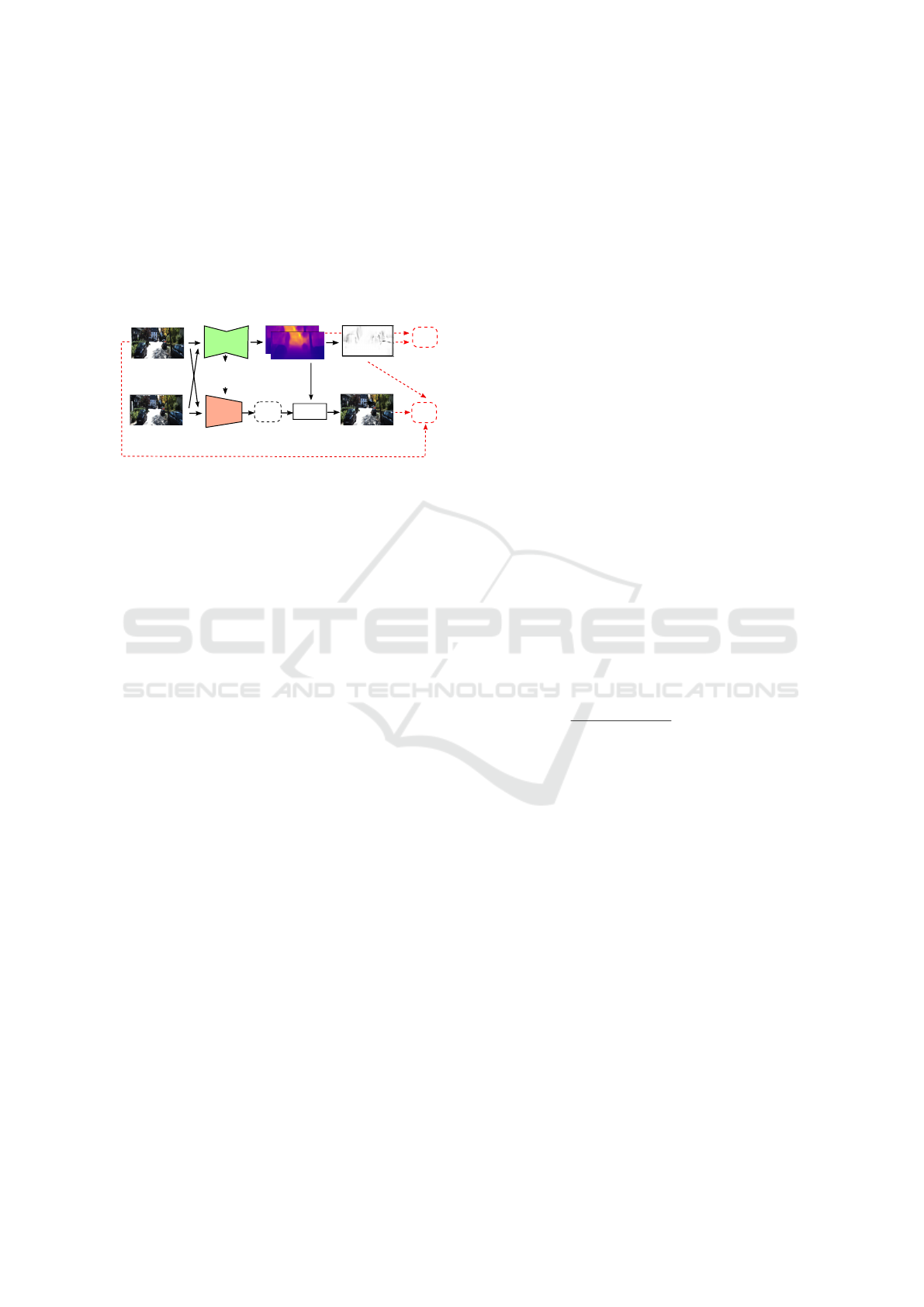
We summarize our method in Figure 1. In this section,
we give an overview of the formulation used for depth
and camera motion estimation. Then, we describe our
geometric consistency constraint and feature sharing
mechanism. Finally, we present architecture consid-
erations of our neural network.
T
t→s
Depth network
Warp
I
s→t
I
s
Feature
Sharing
Soft Visibility
Mask V
t
{D
t,
D
s→t
}
Camera motion
network
L
dc
L
rec
I
t
Figure 1: Overview of our method. The depth network is
used to predict the depth maps for the source I
s
and target I
t
images. The camera motion network predicts the Euclidean
transformation between the target and source camera coor-
dinate systems T
t→s
. A soft-visibility mask is computed
based on the target depth map and the projected source
depth map D
s→t
. Feature maps of the depth network are
shared with the camera motion network. Depth consistency
and reconstruction loss terms are computed considering the
soft visibility mask V
t
.
3.1 Overview
The core idea of self-supervised depth estimation is
that, given two views of the same scene, we can re-
construct one of the views, that is, the target view I
t
,
from the other view, that is, the source view I
s
. Thus,
reconstruction error is used to guide the learning of
the model.
Reconstruction is done through perspective pro-
jection and the relative camera motion between a pair
of views. Perspective projection requires to have the
intrinsic parameters of the camera K, and the depth
values for each pixel in the target image. We obtain
depth values using a convolutional encoder-decoder
network D
θ
that learns to estimate a dense depth map
D for an input image I.
The relative camera motion is represented by an
Euclidean transformation T
t→s
∈ SE(3) between the
coordinate systems that the camera had when the tar-
get view I
t
and the source view I
s
were captured.
Given a pair of views (I
t
, I
s
), we estimate its motion
transformation T
t→s
using a convolutional network
P
φ
.
We reconstruct the target frame by projecting each
pixel coordinate from the target view to the source
view. Given a pixel x
t
in the target frame, its coordi-
nate is back-projected to the camera coordinate sys-
tem of the target view using the inverse of its intrinsic
matrix K
−1
. Then, the relative motion transforma-
tion T
t−>s
is applied to project the coordinates form
the coordinate system of the target view to the coor-
dinate system of the source view. Finally, coordinates
are projected to pixel coordinates on the source view.
Equation 1 shows this mapping:
h(x
s
) = π(KT
t→s
D
t
(x
t
)K
−1
h(x
t
)) (1)
where h(x) is the homogeneous representation of the
pixel x, and π is a function that normalizes homoge-
neous coordinates dividing their values by the last co-
ordinate. The resulting coordinates can be floating
points. Thus, bilinear interpolation is used to com-
pute the pixel intensity values (Zhou et al., 2017). Us-
ing these pixel coordinates and intensity correspon-
dences, we reconstruct the target frame as I
s→t
(x
t
) =
I
s
(x
s
).
Then, we use the reconstruction error for training.
Equation 2 shows the reconstruction loss term.
L
rec
=
∑
I
s
∈{I
t−1
,I
t+1
}
M
t−>s
ρ(I
t
(x
t
), I
s→t
(x
t
)) (2)
We consider the two adjacent frames of the tar-
get as source frames. ρ is a dissimilarity function.
In addition, we use the principled mask M
t−>s
pro-
posed by Mahjourian et al. (2018) to ignore pixels
that became not visible because of the camera mo-
tion. As several works of the literature, we use a com-
posed dissimilarity function that combines the struc-
tural similarity (SSIM) and L1 distance with an α
r
trade-off parameter.
ρ(I
a
, I
b
) = α
r
1 − SSIM(I
a
, I
b
)
2
+(1−α
r
)|I
a
−I
b
| (3)
However, photometric loss is not-informative in
homogeneous regions since in these regions multiple
depth assignments can produce equally good recon-
structions (Garg et al., 2016). This problem can be
addressed by enforcing continuity on depth maps. We
use the edge-preserving local smoothness term used
by Godard et al. (2017) and Yin and Shi (2018).
L
ds
=
∑
x∈Ω(I
t
)
|∇D
t
(x)|(e
|∇I
t
(x)|
)
T
(4)
In addition, the depth network is designed to pre-
dict depth maps at multiple scales to address the gra-
dient locality problem (Zhou et al., 2017; Garg et al.,
2016). Thus, we train the model with the loss function
shown in Equation 5:
L =
∑
i∈S
L
i
rec
+ λ
ds
L
i
ds
(5)
where S is the set of desired scales.
The described considerations are used for our
baseline method. Both the depth network D
θ
and the
camera motion network M
φ
are trained jointly in an
end-to-end manner.
VISAPP 2020 - 15th International Conference on Computer Vision Theory and Applications
136
3.2 Depth Consistency and Occlusion
Depth map and camera motion predictions determine
implicitly a flow field that contains the displacement
of each pixel coordinate from the target frame to the
source frame. This flow field allows us to warp not
only the source frame appearance I
t
but also its dense
depth map D
t
. For instance, we can warp the depth
map of the source frame D
s
to the target frame.
Then, the depth maps predicted for the target
frame D
t
should be consistent with the warped depth
map D
s−>t
. Depth consistency can also be enforced
in the inverse direction, that is, in the forward and
backward direction.
L
dc
=
∑
x∈Ω(I
t
)
|D
t
(x) − D
s−>t
(x)| (6)
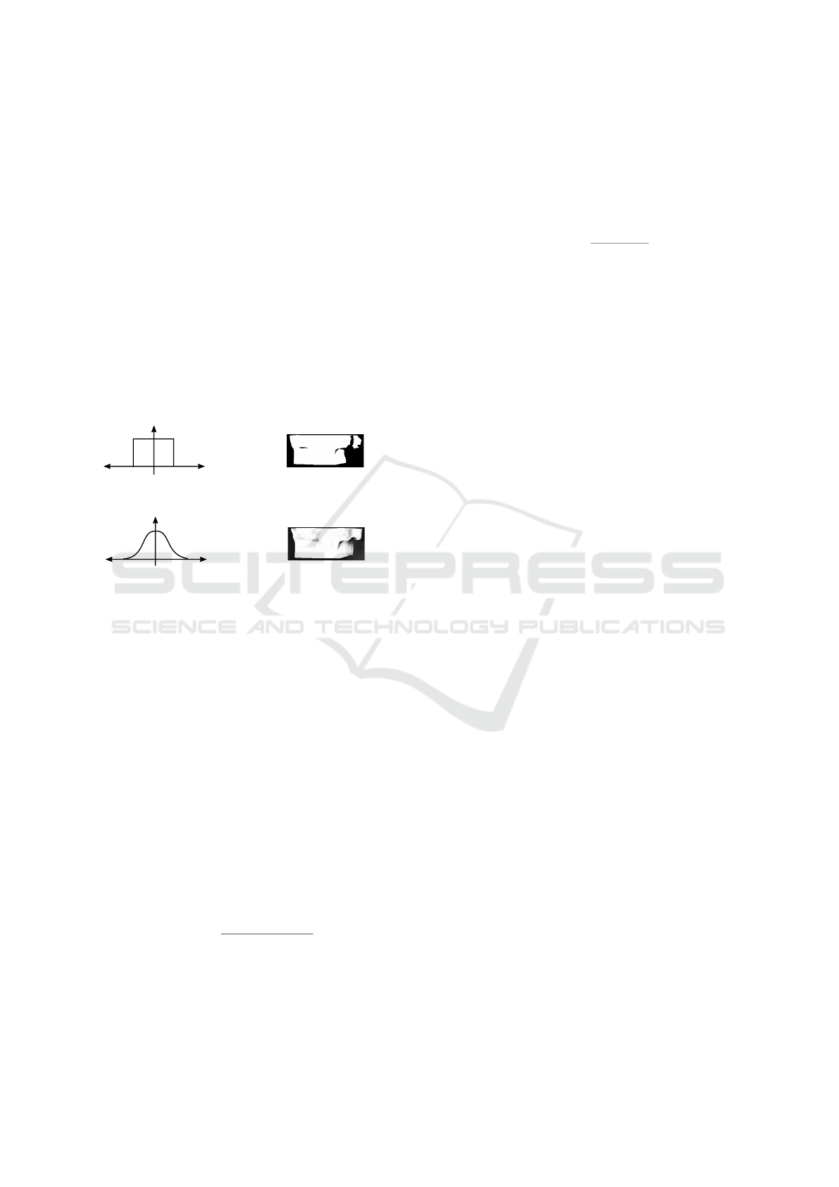
Tresholded visibility mask
Soft-visibility mask
Visibility
Visibility
Depth
difference
Depth
difference
(c)
(b)
(a)
(d)
Figure 2: Thresholded and soft visibility masks. In the first
row, we show the visibility as function of the (a) normalized
depth difference and a (b) sample mask with thresholding.
On the second row, we show the (c) mapping and (d) mask
for the soft-visibility approach.
Depth consistency does not hold for all pixels in
the image because of the occlusions and disocclusions
produced by camera motion or by moving objects in
the scene. Some works use this prior to create a visi-
bility mask that hide or decrease the error contribution
of pixels that have large inconsistencies.
Inconsistency at each pixel in the target image can
be measured as absolute value of normalized differ-
ence between the predicted depth value on the tar-
get image, and the depth value of the source depth
map projected to the target camera coordinate system.
Then, we can compute a visibility mask by threshold-
ing the inconsistencies along the target image with a
threshold t obtained empirically. Equation 7 shows
this relation.
V
t
(x) =
D
t
(x) − D
s→t
(x)
D
t
(x)
< t
(7)
where [.] is the Iverson bracket operator.
However, the networks do not produce accurate
predictions on training, and a constant threshold can-
not handle the inconsistency variability. Thus, instead
ignoring several regions in the reconstruction loss, we
propose to reduce the error contribution of inconsis-
tent regions mapping normalized depth maps differ-
ence to a visibility value using a Gaussian function.
Equation 8 shows the formula of our soft-visibility
mask.
V
t
(x) = e
−α
d
D
t
(x)−D
s→t
(x)
D
t
(x)
2
(8)
where α
d
controls the smoothness degree of the vis-
ibility mask. Figure 2 shows the inconsistency-
visibility and visibility masks obtained with thresh-
olding or with a Gaussian on the inconsistencies.
We apply the visibility mask to the depth consis-
tency and reconstruction loss terms.
L
dc
=
∑
x∈Ω(I
t
)
V
t
(x)|D
t
(x) − D
s−>t
(x)| (9)
L
rec
=
∑
I
s
∈{I
t−1
,I
t+1
}
V
t
M
t−>s
ρ(I
t
(x
t
), I
s→t
(x
t
)) (10)
Thus, Equation 11 denotes our final loss function.
L =
∑
i∈S
L
i
rec
+ λ
ds
L
i
ds
+ λ
dc
L
i
dc
(11)
3.3 Depth Encoder Feature Sharing
It has been shown that using a network with some de-
gree of representation sharing can be better than using
separate networks (Misra et al., 2016; Doersch and
Zisserman, 2017; Liu et al., 2019), mainly because
individual tasks can be reinforced with the represen-
tation of other tasks and also because feature sharing
allows representations to avoid over-fitting in individ-
ual tasks, but to be useful in other tasks.
In our context, where estimation of depth and
camera motion operates simultaneously with the same
input data and where tasks are complementary be-
cause the geometric formulation provides supervision
to both networks with the same loss function, this mo-
tivates us to believe that representation sharing can
improve the model performance.
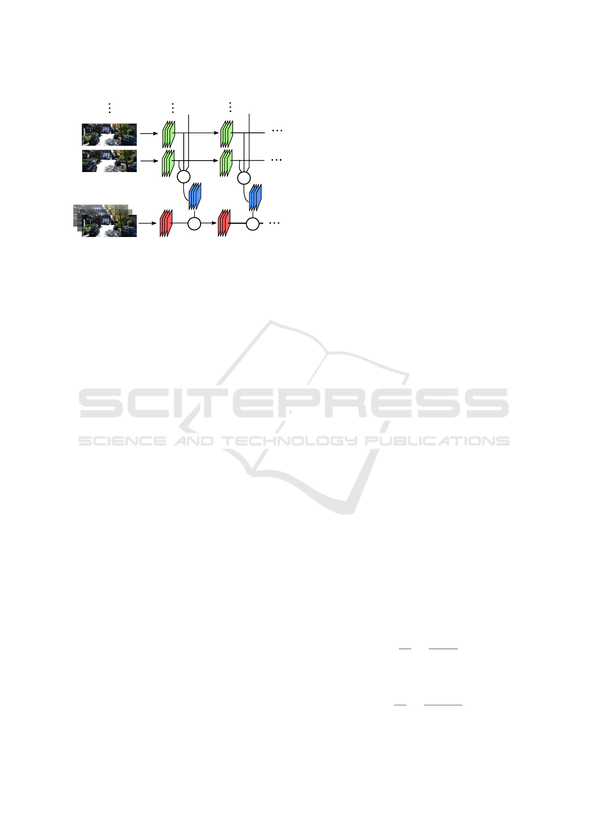
Figure 3 illustrates our feature attention mecha-
nism. We propose to share the feature maps of the
depth encoder with the pose network. This allows
the pose network to leverage the depth features to im-
prove the pose estimation. Moreover, better pose esti-
mates can potentially improve the reconstruction and,
as a consequence, depth estimation.
Equation 12 summarizes our proposal. Given a
target frame I
t
and its source frames I
t−1
and I
t+1
,
our depth network produces feature maps from these
frames at each layer of the network. Thus, F
l
t
, F
l
t−1
,
and F
l
t+1
are the features on the layer l for the tar-
get and source frames, respectively. In addition, we
Self-supervised Depth Estimation based on Feature Sharing and Consistency Constraints
137
C
f
+
C
F
P
f
F
D
t-1
F
P
F
PD
F
PD
1
F
D
t+1
2
1 2
2
1
F
D
t-1
F
D
t+1
2
1
F
D
t
1
F
D
t
2
+
Figure 3: Feature sharing mechanism. The feature maps in
the depth and camera motion network are shown with green
and red colors, respectively. ”C” represents the concatena-
tion operation. f is a function that transforms the concate-
nated depth features. ”+” represents the element-wise sum
operation.
apply a non-linear transformation f over the concate-
nated depth representations. For simplicity, we set f
to be convolution layer with 1x1 filters. We set the
output of f to have the same amount of feature maps
of the pose network in the same layer level. Finally,
we sum the transformed features to the pose features.
F
l
PD
= F
l
P
+ f ([F
l
D
t
: F
l
D
t−1
: F
l
D
t+1
]) (12)
3.4 Network Architecture
Finally, we briefly describe the network architecture.
Our depth encoder-decoder network is based on the
DepthNet (Yin and Shi, 2018). Its encoder network
is based on the ResNet50. Its decoder network is
composed of deconvolutional layers that up-sample
the bottleneck representation in order to upscale the
feature maps to the input resolution.
The encoder network has skip connections with
the decoder network. In addition, we use dropout af-
ter the last two layers of the encoder and the first two
of the decoder network to reduce over-fitting. In ad-
dition, we use bilinear interpolation for up-sampling
instead of nearest-neighbor interpolation to produce
more accurate depth maps.
Our camera motion network predicts the relative
motion between two input frames. The relative cam-
era motion has a 6-DoF representation, that is, the ro-
tation angles and the translation vectors. We use the
architecture proposed by Zhou et al. (2017).
4 EXPERIMENTS
In this section, we describe and evaluate the experi-
mental results achieved with the proposed method.
4.1 Experimental Setup
In this section, we describe the parameters of our
model and the optimization method used in the learn-
ing process, the dataset used for training and evaluat-
ing the models and, finally, the metrics used to assess
the model performance.
4.1.1 Parameter Setup
We used a trade-off parameter α
r
= 0.85 in the recon-
struction loss term. The weights of the depth smooth-
ness λ
ds
and depth consistency terms λ
dc
are 0.5 and
0.31, respectively. We employed a smoothness pa-
rameter of the visibility map α
d
= 2. We used a
threshold t = 0.3 for the alternative version of our
method with the thresholded visibility mask. We ap-
plied Adam optimization with parameter β
1
= 0.9 and
β
2
= 0.999. We chose a batch size of 4.
The input images are re-scaled to 128×416. Fur-
thermore, we apply random scaling, cropping, and
various color perturbations to the input images in the
data augmentation stage to reduce over-fitting. Depth
and camera motion networks are trained from scratch.
4.1.2 Dataset
We used the KITTI 2015 dataset, composed of video
sequences with 93 thousand images acquired by RGB
cameras, and with sparse depth ground-truth provided
by Velodyne LIDAR scanner.
As several works available in the literature, we
used the Eigen split (Eigen et al., 2014) for evalua-
tion. It contains 40K images for training, 4K images
for validation, and 687 images for testing.
4.1.3 Metrics
We used the standard metrics used in other methods
available in the literature, described as follows:
• absolute relative difference:
E =
1
|T |
∑
y∈T
|y − y
∗
|
y
∗
(13)
• squared relative difference:
E =
1
|T |
∑
y∈T
||y − y
∗
||
2
y
∗
(14)
VISAPP 2020 - 15th International Conference on Computer Vision Theory and Applications
138
• root mean squared error:
E =
s
1
|T |
∑
y∈T
||y − y
∗
||
2
(15)
• log root mean squared error:
E =
s
1
|T |
∑
y∈T
||logy − log y
∗
||
2
(16)
where y and y∗ are the predicted and ground-truth
depth values, and T represents the sets of pixels in
the image with depth ground-truth.
Moreover, we used the thresholded accuracy met-
ric, which is the proportion of depth values with a
ratio of the predicted to ground-truth value in the in-
terval <
1
δ
, δ >. Similar to previous works, we com-
puted the proportion for the intervals defined by δ val-
ues equal to 1.25, 1.25
2
and 1.25
3
.
E =
1
|T |
∑
y∈T
[max(
y
y
∗
,
y
∗
y
) < δ] (17)
where [.] is the Iverson bracket operator.
4.2 Depth Estimation
In this section, we present our experiments. First,
we perform ablative experiments to analyze the im-
pact of each contribution on the performance of our
model. Then, we compare our results with other self-
supervised depth estimation methods categorized into
three groups: methods that assume a static scene,
methods that explicitly model moving objects on the
scene, and methods that perform parameter or output
fine-tuning at test time.
4.2.1 Ablation Study
Table 1 shows the performance of variants of our
model. It is possible to observe that the addition of
depth consistency and either a hard or soft visibility
masks is the major source of improvement. More-
over, we can see that the soft visibility map is slightly
better than the thresholded visibility mask. It is also
possible to observe that the complete model obtains
better results than just considering depth consistency
and visibility mask.
4.2.2 State-of-the-Art Comparison
Table 2 shows our results compared with the state-of-
the-art methods. Methods of the literature categorized
into three groups. First, we show that our method out-
performed the competing methods that assume a rigid
scene with almost all metrics. In addition, we show
that our method obtained competitive results when
compared with methods that explicitly address mov-
ing objects. Finally, we show that our method did not
outperform results obtained with methods in the lit-
erature that explicitly model moving objects and per-
form test-time fine-tuning.
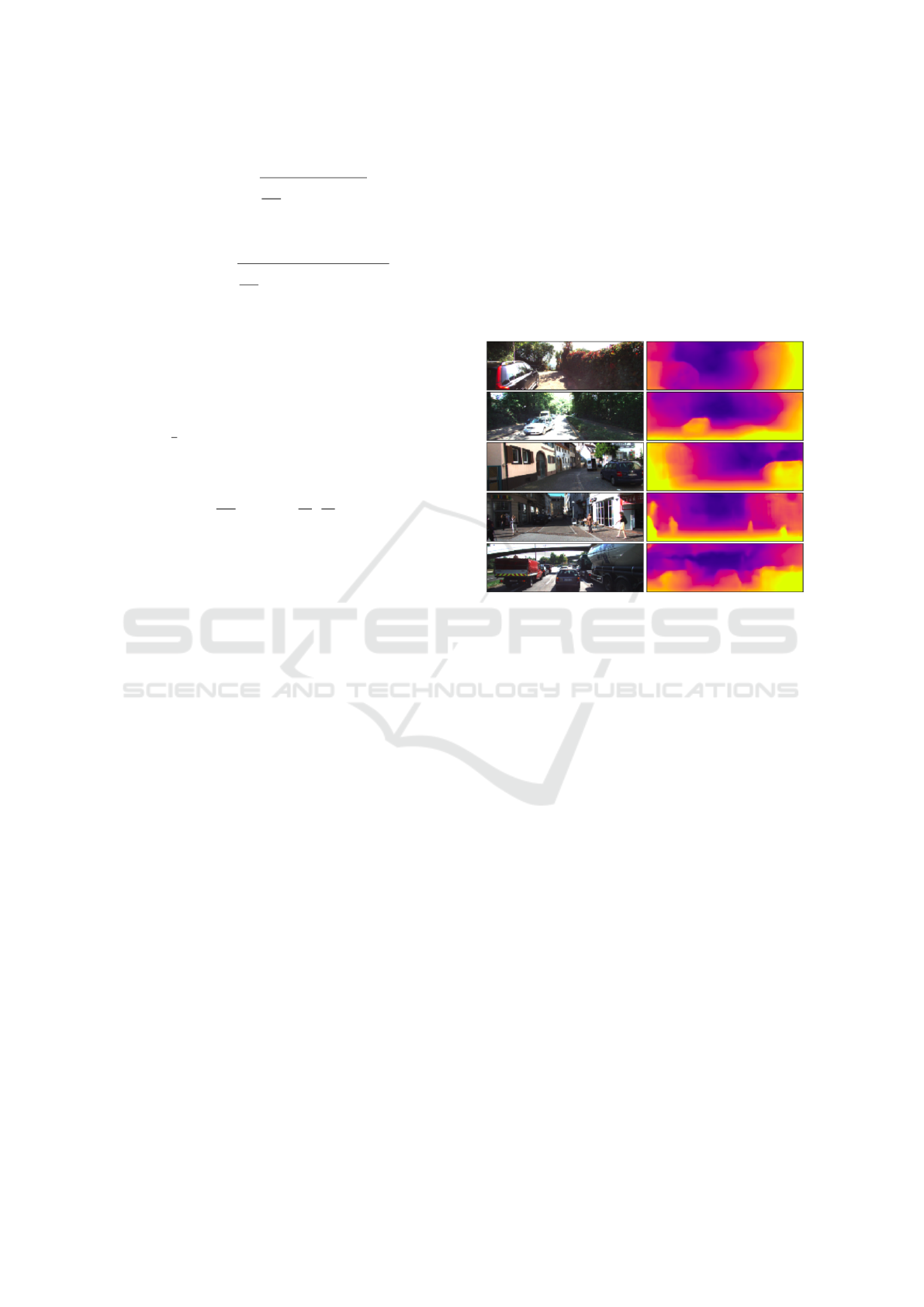
Figure 4 shows that depth maps predicted through
our method can capture the structure of the scene.
In addition, the last two images show that, when the
scene is not rigid, our method is more prone to errors.
Figure 4: Input images and corresponding depth maps pro-
duced with our method. Images were sampled from the
KITTI dataset.
5 CONCLUSIONS
We proposed a self-supervised method for monocular
depth estimation that relies on (i) a depth consistency
constraint, (ii) a soft visibility map that reduces the er-
ror contribution in depth inconsistent regions, and (iii)
sharing features from the depth to the camera motion
networks.
We showed that depth consistency constraint and
feature sharing can improve the performance of our
baseline model and become competitive even with
methods that explicitly model moving objects in the
scene.
ACKNOWLEDGEMENTS
The authors are thankful to FAPESP (grants
#2017/12646-3 and #2018/00031-7), CNPq (grants
#305169/2015-7 and #309330/2018-7) and CAPES
for their financial support. They are also grateful to
NVIDIA Corporation for the donation of a GPU as
part of the GPU Grant Program.
Self-supervised Depth Estimation based on Feature Sharing and Consistency Constraints
139

Table 1: Ablation analysis. We show the results of various alternative models. First, we show that our baseline model obtained
poor results. Then, we show that the addition of depth consistency (DC) and thresholded visibility mask (TV) improved the
performance of our model. Furthermore, we show that the use of the soft visibility mask (SV) increased our results in almost
all the evaluation metrics. Finally, we show results achieved with our final model through depth consistency, soft visibility
mask and feature sharing (FS). The best result achieved for each metric is highlighted in bold.
Method
Lower is better Higher is better
Abs Rel Sq Rel RMSE Log RMSE δ = 1.25 δ = 1.25
2
δ = 1.25
3
Baseline 0.150 1.266 5.864 0.232 0.803 0.932 0.973
Ours w/ DC & TV, w/o FS 0.141 1.061 5.679 0.222 0.809 0.936 0.976
Ours w/ DC & SV, w/o FS 0.141 1.029 5.536 0.219 0.811 0.939 0.977
Ours 0.138 1.030 5.394 0.216 0.820 0.941 0.977
Table 2: Results of depth estimation on the Eigen split of the KITTI dataset. We compare our results against several methods
of the literature. Methods are categorized into three groups: methods that assume rigid scenes, methods that explicitly model
moving objects, and methods that perform fine-tuning on the last layer of the network besides considering moving objects. (*)
indicates newly results obtained from an official repository. Column ”M” indicates whether the method has address moving
objects explicitly. Column ”F” indicates whether the method performs test-time fine-tuning. The best result achieved for each
metric is highlighted in bold.
Method
Lower is better Higher is better
Abs Rel Sq Rel RMSE Log RMSE δ = 1.25 δ = 1.25
2
δ = 1.25
3
M. F.
Zhou et al. (2017)* 0.183 1.595 6.709 0.270 0.734 0.902 0.959
Mahjourian et al. (2018) 0.163 1.240 6.220 0.250 0.762 0.916 0.967
Wang et al. (2018) 0.151 1.257 5.583 0.228 0.810 0.936 0.974
Yin and Shi (2018)* 0.149 1.060 5.567 0.226 0.796 0.935 0.975
Zou et al. (2018) 0.150 1.124 5.507 0.223 0.806 0.933 0.973
Almalioglu et al. (2019) 0.150 1.141 5.448 0.216 0.808 0.939 0.975
Zhou et al. (2018) ”LR” 0.143 1.104 5.370 0.219 0.824 0.937 0.975
Ours 0.138 1.030 5.394 0.216 0.820 0.941 0.977
Luo et al. (2018) 0.141 1.029 5.350 0.216 0.816 0.941 0.976 3
Ranjan et al. (2019) 0.140 1.070 5.326 0.217 0.826 0.941 0.975 3
Ours 0.138 1.030 5.394 0.216 0.820 0.941 0.977
Casser et al. (2019) ”M” 0.141 1.026 5.290 0.215 0.816 0.945 0.979 3
Gordon et al. (2019) 0.128 0.959 5.230 0.212 0.845 0.947 0.976 3
Ours 0.138 1.030 5.394 0.216 0.820 0.941 0.977
Casser et al. (2019) ”M + R” 0.109 0.825 4.750 0.187 0.874 0.958 0.983 3 3
Chen et al. (2019) 0.099 0.796 4.743 0.186 0.884 0.955 0.979 3 3
REFERENCES
Almalioglu, Y., Saputra, M. R. U., de Gusmao, P. P.,
Markham, A., and Trigoni, N. (2019). GANVO:
Unsupervised Deep Monocular Visual Odometry and
Depth Estimation with Generative Adversarial Net-
works. In International Conference on Robotics and
Automation, pages 5474–5480. IEEE.
Casser, V., Pirk, S., Mahjourian, R., and Angelova,
A. (2019). Depth Prediction without the Sensors:
Leveraging Structure for Unsupervised Learning from
Monocular Videos. In AAAI Conference on Artificial
Intelligence, volume 33, pages 8001–8008.
Chen, Y., Schmid, C., and Sminchisescu, C. (2019). Self-
Supervised Learning with Geometric Constraints in
Monocular Video: Connecting Flow, Depth, and
Camera. arXiv preprint arXiv:1907.05820.
Concha, D., Maia, H., Pedrini, H., Tacon, H., Brito, A.,
Chaves, H., and Vieira, M. (2018). Multi-Stream Con-
volutional Neural Networks for Action Recognition in
Video Sequences Based on Adaptive Visual Rhythms.
In 17th IEEE International Conference on Machine
Learning and Applications, pages 473–480, Orlando-
FL, USA.
Doersch, C. and Zisserman, A. (2017). Multi-Task Self-
Supervised Visual Learning. In IEEE International
Conference on Computer Vision, pages 2051–2060.
Eigen, D., Puhrsch, C., and Fergus, R. (2014). Depth Map
Prediction from a Single image using a Multi-Scale
Deep Network. In Advances in Neural Information
VISAPP 2020 - 15th International Conference on Computer Vision Theory and Applications
140

Processing Systems, pages 2366–2374.
Garg, R., BG, V. K., Carneiro, G., and Reid, I. (2016). Un-
supervised CNN for Single View Depth Estimation:
Geometry to the Rescue. In European Conference on
Computer Vision, pages 740–756. Springer.
Godard, C., Mac Aodha, O., and Brostow, G. J. (2017).
Unsupervised Monocular Depth Estimation with Left-
Right Consistency. In IEEE Conference on Computer
Vision and Pattern Recognition, pages 270–279.
Gordon, A., Li, H., Jonschkowski, R., and Angelova, A.
(2019). Depth from Videos in the Wild: Unsupervised
Monocular Depth Learning from Unknown Cameras.
arXiv preprint arXiv:1904.04998.
Lee, M. and Fowlkes, C. C. (2019). CeMNet: Self-
Supervised Learning for Accurate Continuous Ego-
motion Estimation. In IEEE Conference on Computer
Vision and Pattern Recognition Workshops, pages 0–
0.
Li, R., Wang, S., Long, Z., and Gu, D. (2018). Undeepvo:
Monocular Visual Odometry through Unsupervised
Deep Learning. In IEEE International Conference on
Robotics and Automation, pages 7286–7291. IEEE.
Liu, S., Johns, E., and Davison, A. J. (2019). End-to-End
Multi-Task Learning with Attention. In IEEE Con-
ference on Computer Vision and Pattern Recognition,
pages 1871–1880.
Luo, C., Yang, Z., Wang, P., Wang, Y., Xu, W., Nevatia, R.,
and Yuille, A. (2018). Every Pixel Counts++: Joint
Learning of Geometry and Motion with 3D Holistic
Understanding. arXiv preprint arXiv:1810.06125.
Mahjourian, R., Wicke, M., and Angelova, A. (2018). Un-
supervised Learning of Depth and Ego-motion from
Monocular Video using 3D Geometric Constraints.
In IEEE Conference on Computer Vision and Pattern
Recognition, pages 5667–5675.
Misra, I., Shrivastava, A., Gupta, A., and Hebert, M. (2016).
Cross-Stitch Networks for Multi-Task Learning. In
IEEE Conference on Computer Vision and Pattern
Recognition, pages 3994–4003.
Pillai, S., Ambrus¸, R., and Gaidon, A. (2019). Superdepth:
Self-Supervised, Super-Resolved Monocular Depth
Estimation. In International Conference on Robotics
and Automation, pages 9250–9256. IEEE.
Ranjan, A., Jampani, V., Balles, L., Kim, K., Sun, D., Wulff,
J., and Black, M. J. (2019). Competitive Collabo-
ration: Joint Unsupervised Learning of Depth, Cam-
era Motion, Optical Flow and Motion Segmentation.
In IEEE Conference on Computer Vision and Pattern
Recognition, pages 12240–12249.
Ruder, S., Bingel, J., Augenstein, I., and Søgaard, A.
(2017). Latent Multi-Task Architecture Learning.
arXiv preprint arXiv:1705.08142.
Santos, A. and Pedrini, H. (2019). Spatio-Temporal Video
Autoencoder for Human Action Recognition. In 14th
International Joint Conference on Computer Vision,
Imaging and Computer Graphics Theory and Appli-
cations, pages 114–123, Prague, Czech Republic.
Souza, M., Fonseca, L., and Pedrini, H. (2018). Im-
provement of Global Motion Estimation in Two-
Dimensional Digital Video Stabilization Methods.
IET Image Processing, 12(12):2204–2211.
Tacon, H., Brito, A., Chaves, H., Vieira, M., Villela, S.,
Maia, H., Concha, D., and Pedrini, H. (2019). Hu-
man Action Recognition Using Convolutional Neural
Networks with Symmetric Time Extension of Visual
Rhythms. In 19th International Conference on Com-
putational Science and its Applications, pages 351–
366, Saint Petersburg, Russia.
Triggs, B., McLauchlan, P. F., Hartley, R. I., and Fitzgibbon,
A. W. (1999). Bundle Adjustment: A Modern Synthe-
sis. In International Workshop on Vision Algorithms,
pages 298–372. Springer.
Wang, C., Miguel Buenaposada, J., Zhu, R., and Lucey, S.
(2018). Learning Depth from Monocular Videos using
Direct Methods. In IEEE Conference on Computer
Vision and Pattern Recognition, pages 2022–2030.
Xu, H., Zheng, J., Cai, J., and Zhang, J. (2019). Region
Deformer Networks for Unsupervised Depth Estima-
tion from Unconstrained Monocular Videos. arXiv
preprint arXiv:1902.09907.
Yin, Z. and Shi, J. (2018). Geonet: Unsupervised Learn-
ing of Dense Depth, Optical Flow and Camera Pose.
In IEEE Conference on Computer Vision and Pattern
Recognition, pages 1983–1992.
Zhou, L., Ye, J., Abello, M., Wang, S., and Kaess,
M. (2018). Unsupervised Learning of Monoc-
ular Depth Estimation with Bundle Adjustment,
Super-Resolution and Clip Loss. arXiv preprint
arXiv:1812.03368.
Zhou, T., Brown, M., Snavely, N., and Lowe, D. G.
(2017). Unsupervised Learning of Depth and Ego-
Motion from Video. In IEEE Conference on Computer
Vision and Pattern Recognition, pages 1851–1858.
Zou, Y., Luo, Z., and Huang, J.-B. (2018). Df-Net: Un-
supervised Joint Learning of Depth and Flow using
Cross-Task Consistency. In European Conference on
Computer Vision, pages 36–53.
Self-supervised Depth Estimation based on Feature Sharing and Consistency Constraints
141
