Deviation Prediction and Correction on Low-Cost Atmospheric

Pressure Sensors using a Machine-Learning Algorithm

Tiago C. de Araújo

, Lígia T. Silva

and Adriano J. C. Moreira

Algoritmi Research Centre, Universidade do Minho, Guimarães, Portugal

CTAC Research Centre, Universidade do Minho, Guimarães, Portugal

Keywords: Low-Cost Sensors, Data Quality, Machine Learning, Environmental Monitoring, Collaborative Sensing.

Abstract: Atmospheric pressure sensors are important devices for several applications, including environment

monitoring and indoor positioning tracking systems. This paper proposes a method to enhance the quality of

data obtained from low-cost atmospheric pressure sensors using a machine learning algorithm to predict the

error behaviour. By using the extremely Randomized Trees algorithm, a model was trained with a reference

sensor data for temperature and humidity and with all low-cost sensor datasets that were co-located into an

artificial climatic chamber that simulated different climatic situations. Fifteen low-cost environmental sensor

units, composed by five different models, were considered. They measure – together – temperature, relative

humidity and atmospheric pressure. In the evaluation, three categories of output metrics were considered:

raw; trained by the independent sensor data; and trained by the low-cost sensor data. The model trained by

the reference sensor was able to reduce the Mean Absolute Error (MAE) between atmospheric pressure sensor

pairs by up to 67%, while the same ensemble trained with all low-cost data was able to reduce the MAE by

up to 98%. These results suggest that low-cost environmental sensors can be a good asset if their data are

properly processed.

1 INTRODUCTION

Low-cost environmental sensors have enabled

individuals to build and manage their own monitoring

system not only by its lower price, but also due to its

easy availability and extended technical support.

Therefore, when engaged individuals share a

common concern, such as the quality of the

environment, those particular monitoring artefacts,

together, can be part of a collaborative monitoring

system (Goldman et al., 2009; Zaman et al., 2014).

Collaborative sensing, either mobile or not, can be

helpful as a complementary tool in several fields of

study, such as biology (Kanhere, 2011), urban

environment and weather and local climate (D’Hondt

et al., 2013; Young et al., 2014).

The use of such sensors can help to reduce overall

costs to maintain an urban environmental monitoring

system in continuous run. A specific concern about

urban areas is the urban heat islands. The continuous

https://orcid.org/0000-0002-1766-5768

https://orcid.org/0000-0002-0199-8664

https://orcid.org/0000-0002-8967-118X

monitoring of environmental conditions in urban

areas can help in the assessment and in triggering

actions towards prevention or mitigation of urban

heat islands as demonstrated by (Magli et al., 2016;

Qaid et al., 2016; Salata et al., 2017) or other human-

caused local phenomena, such as air pollution.

The study of air quality is another field that has

also seen an increase in the utilization of low-cost

sensors (Kumar et al., 2015). As an example, the

authors in (Hu et al., 2016) described the design and

evaluation of an air-quality monitoring system that

uses low-cost sensors and found the performance of

the sensors to be satisfactory; the authors in (Duvall

et al., 2016) investigated the performance of low-cost

sensors for ozone and nitrogen dioxide monitoring

and its application in a community, and found that the

sensors, handled by citizen scientists, provided

consistent and positive readings in most of the

situations. Once the sensors are evaluated positively,

they can feed, for example, a local air quality

evaluation system as described by (Silva & Mendes,

de Araújo, T., Silva, L. and Moreira, A.

Deviation Prediction and Correction on Low-Cost Atmospheric Pressure Sensors using a Machine-Learning Algorithm.

DOI: 10.5220/0008968400410051

In Proceedings of the 9th International Conference on Sensor Networks (SENSORNETS 2020), pages 41-51

ISBN: 978-989-758-403-9; ISSN: 2184-4380

2012). In an indoor scenario, they can also be used for

air-quality assessment by monitoring the levels of

, once it has relevant consequences on cognitive

performance of the occupants, as described by (Allen

et al., 2016; Satish et al., 2012). They can even be

used as a complementary asset for indoor surveillance

(Szczurek et al., 2017).

Electronic sensors are often controlled by

hardware with embedded microprocessors, such as

Arduino, Raspberry Pi or NodeMCU. Amongst these,

Arduino is, perhaps, the most popular among non-

specialized users in a citizen science scope. Several

works about Internet of Things, Environmental

Monitoring and Sensor Evaluations used Arduino as

a platform for data collection due to its ease of use

and widespread collaborative support (de Araújo et

al., 2017; Fuertes et al., 2015; Piedrahita et al., 2014;

Saini et al., 2016; Sinha et al., 2015; Trilles et al.,

2015).

However, low-cost environmental sensors cannot

be deployed into the field without minimal

verifications regarding their data-quality, even when

nominally calibrated from factory. Afterall, the value

of a running sensing system is strictly related to the

quality of its data, as scrutinized by (Liu et al., 2015).

Data quality assessment, by itself, is a difficult task,

mostly because bad quality data can be originated

from diverse sources, including a bad sensor

behaviour (Gitzel, 2016). In air quality studies, the

investigators in (Borrego et al., 2016) studied the data

quality of microsensors by comparison with reference

methods for air quality monitoring. They found that

the performance can vary from one sensor to another,

even if being of the same type. With similar results,

authors in (Castell et al., 2017) found that low-cost

sensors, despite its issues on reproducibility, can

provide very good data for lower-tie applications,

such as pollution awareness and environmental

monitoring in a coarse scale. However, improvements

are necessary if the goal is a high-accuracy

application.

Authors in (Terando et al., 2017) and (Ashcroft,

2018) discussed the errors involved in environmental

monitoring with microsensors and professional

stations. They pointed out that both approaches may

not differ in terms of error sources, since biased

temperature readings may be common in both

situations due to the lack of standardization on

thermal shields and positioning. However, despite the

technical issues involved in temperature monitoring,

the author in (Mwangi, 2017) demonstrated the

importance of low-cost sensors for building weather

stations in developing countries, places without

sufficient resources for conventional monitoring. In

the reported experiment, the sensors were first

calibrated by placing the low-cost monitoring station

close to reference instruments and, then, the artefacts

were deployed into the field, achieving good results.

The use of barometric pressure sensors in weather

monitoring is important since pressure is a good

predictor for rainfall, as it is closely related to water

evaporation rate (Özgür & Koçak, 2015). In simple

terms, low pressure values, compared to typical

values, may indicate rain, whereas high pressure

values may indicate clean weather. Beyond

environmental monitoring, atmospheric pressure has

also great importance for medical applications,

automotive industry and positioning estimation for

mobile computing (Yunus et al., 2015). In indoor and

outdoor positioning systems, barometric pressure can

provide a good estimate of altitude, since the air

pressure value is about 1013hPa at sea-level and, it

drops by approximately 0.11hPa per meter in the first

1000 meters of altitude. Thus, the enhancement of

data quality in these sensors may empower its use for

several applications.

Machine learning has also attracted the attention

of non-specialized users in citizen science projects.

Some contributing factors to its spreading are its

accessibility through built-in open-source packages,

such as “scikit-learn” for Python programming

language (Scikit-Learn, 2019), and the available

tutorials and collaborative support by other users

through web communities such as GitHub, Quora and

StackExchange. Machine learning algorithms can be

applied to sensor analysis as a powerful calibration

tool. Authors in (Yamamoto et al., 2017) used a

machine learning-based model for calibration of

temperature sensors in outdoor monitoring, and

reduced the errors of subject sensors satisfactorily.

For air quality applications, the authors in

(Zimmerman et al., 2018) used Random Forest

ensemble as a regressor between multidimensional

data for air-pollutant sensors, including cross-

sensitivity. They reached the US EPA

recommendations for air quality with the calibrated

low-cost sensors (US-EPA, 2019), highlighting a

promising strategy to overcome poor data, commonly

found in low-cost air quality sensors.

2 RESEARCH PROBLEM AND

APPROACH

The work described in this paper is part of a research

project about the use of low-cost environmental

sensors for monitoring and characterization of urban

SENSORNETS 2020 - 9th International Conference on Sensor Networks

spaces. Its main concern is the data quality obtained

from low-cost sensors.

The most common physical quantities observed in

environmental monitoring are air temperature,

relative humidity and atmospheric pressure. Sensors

involved in the monitoring of these quantities can

often have heterogeneous accuracy, with humidity

and pressure readings being dependent, at least, on

the temperature at which the readings were taken.

Therefore, the errors associated to the readings of a

sensor might be a function of other parameters.

Regarding the atmospheric pressure sensors, as

their transduction principle relies on the surface

deformation of the sensing element due to the

surrounding air pressure, as described by (Minh-

Dung et al., 2013), it is expected that both

temperature and humidity interfere with the sensor

readings.

These considerations lead to the hypothesis that

the errors, or deviations, from atmospheric pressure

sensor readings can be mathematically modeled from

temperature and humidity readings.

We propose the use of a supervised machine

learning algorithm in the modelling process, as

current available regressor algorithms have been

shown to be very effective in solving problems using

both linear and non-linear approximations. The

chosen machine-learning algorithm for the prediction

of errors in atmospheric pressure readings was the

Extremely Randomized Trees (Extra-trees) ensemble

regressor, first proposed by (Geurts et al., 2006), and

available in “sklearn” library for Python 3.7. This

algorithm is suitable for both linear and non-linear

systems with good accuracy and computational

efficiency.

In short terms, in the learning process the

algorithm requires both input and target vectors, so it

can “learn” the behaviour of the output (target) from

the given inputs. Once the model is trained, it can

either provide outputs using new inputs (data that

were not passed in the training process) or correct the

whole existing dataset, by feedback, to assess the

algorithm’s performance in the error prediction.

In the present approach, the input data is

composed by the temperature and humidity readings,

obtained from a set of sensors co-located and

submitted to the same environmental conditions. In

the final dataset each individual sensor data is

represented by a vector (or feature), that, together,

formed a matrix “m x n”, where “m” is the number

of reading samples (the vector length), and “n” is the

number of sensors. The target vector was obtained

from the deviations between a pair of pressure

sensors, point to point, where one of them was

considered as a beacon (a reference). Both data were

merged and then used in the training process.

Consequently, once trained, the model was able to

predict the errors between the atmospheric pressure

sensors using the temperature and humidity data as

input. The predicted error was added back into the

original pressure sensor dataset to, finally, obtain its

corrected readings.

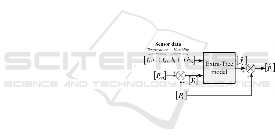
The overall process is illustrated in Figure 1, in

which: “t

, (…), t

” are vectors containing the

temperature readings from “N

” different sensors;

“h

, (…), h

” are vectors containing the humidity

sensor readings from “N

” different sensors; “p

ref

” is

the vector containing the readings from atmospheric

pressure sensor used as reference; “p

” is the vector

containing the readings from a given atmospheric

pressure sensor “i” which will have its readings

adjusted; “y

” is the actual error between the given

sensors (used only in the learning process); “y



” is the

output vector of the model, containing the predicted

error (a function of temperature and humidity); and,

finally, “p



” is the vector containing the corrected

atmospheric pressure sensor readings. All vectors

have length “m”.

Figure 1: Diagram of the approach adopted to predict and

correct deviations between atmospheric pressure sensors.

Moreover, machine-learning algorithms often

allow the adjustment of internal parameters that affect

its performance. The main adjustable parameters for

performance tuning in the Extra-Trees ensemble

regressor are the number of trees in the forest and the

maximum number of split nodes in the decision trees

(this last is used only in classification problems). The

choice of the number of trees has a trade-off: higher

number of trees results in better accuracy but requires

more computational resources. Usually, the default

value for this parameter is “100” and is often used as

a starting value. In case of eventual unsatisfactory

performance, it could be increased or decreased in a

fine-tuning process.

The next section contains the experimental

description that generated the datasets used in the

current investigation.

Deviation Prediction and Correction on Low-Cost Atmospheric Pressure Sensors using a Machine-Learning Algorithm

3 EXPERIMENTAL

The datasets used in this study were obtained from

sensors submitted to controlled conditions inside an

artificial climatic chamber (Aralab Fitoclima®) that

followed a set of instructions to create different

temperature and humidity combinations. The

following sections describe the preparation of the

sensor sets and the experimental execution plan for

the artificial climatic chamber.

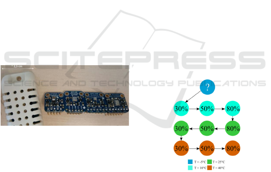
3.1 Sensor Selection and Preparation

Five different models of sensors were chosen due to

its price, availability and ease of use (presence of

built-in interface): AM2302 (Adafruit, 2016),

HTU21D (Measurement Specialties Inc., 2013),

BMP180 (Bosch Sensortec, 2013), BME280 (Bosch

Sensortec, 2015) and MPL3115A2 (Freescale

Semiconductor, 2013) (Figure 2). From these, the

BME280 provides temperature, humidity and

pressure data; AM2302 and HTU21D provide

temperature and humidity data; BMP180 and

MPL3115A2 provide temperature and pressure data.

Three units of each sensor model were used, forming

three sets containing one unit from each sensor model

(identified as Set A, Set B and Set C).

Figure 2: Low-cost sensors selected for the experiment.

From left to right: AM2302, HTU21D, BMP180, BME280

and MPL3115A2.

Each experimental set was assembled around one

Arduino device, equipped with a “SD&RTC” shield

for datalogging with timestamps. There were no

physical relevant spacing between sensors, so they

could read the same quantity values. The sampling

rate was set to one sample per minute.

An additional independent sensor from Lascar

Electronics© (Lascar Electronics, n.d.), factory-

calibrated for temperature and humidity, was also

placed together with the low-cost sensor sets inside

the chamber. Its function was to provide reference

data for later processing and to enable the comparison

of the deviation prediction performances between the

model trained with all sensors and the model trained

only with reference data. Every device was timely

synchronized to avoid reading displacements

between datasets.

3.2 Artificial Climatic Chamber

Configuration

Two experimental profiles were programmed into the

climatic chamber. The first one was programmed

with temperature levels of -5°C, 10°C, 25°C and

40°C; humidity levels of 30%, 50% and 80%. The

total experiment length was 46 hours, including: 11.5

hours for each temperature level in stability; 3 hours

for each humidity level in stability. The second

experimental profile was set by removing the

negative temperature from the first profile and

equally extending the times of each steady level. This

was performed to increase the stability time of

relative humidity and consequently reduce eventual

noise in this quantity.

The programmed execution started at the lowest

value of temperature and ended at the highest. The

relative humidity level sequence followed the scheme

presented in Figure 3. Note that, in the used chamber,

it was not possible to control relative humidity below

0°C. The readings during transitions – either

temperature or humidity – are also of interest and

were considered.

Figure 3: Temperature and humidity sequences

programmed into the artificial climatic chamber.

Those levels were chosen to attempt to cover

typical conditions of an urban environment that does

not experience extreme weather conditions.

Consequently, it should allow the assessment of the

data quality of the low-cost sensors in short-term

timespan within the given hypothetic scenario. After

the execution of all the experiments, more than 560

hours of continuous controlled readings of

SENSORNETS 2020 - 9th International Conference on Sensor Networks

temperature and humidity were obtained, as well as

corresponding readings of the natural atmospheric

pressure (uncontrolled), since the chamber is not

sealed.

The final dataset, generated by joining all the data

gathered from each experiment, consisted of eleven

features (columns) separated by sensor models for the

different physical quantities (with no distinction

between different sensor sets): five for temperature

and three for humidity, used entirely in the training,

and three for atmospheric pressure that were used to

form the error vectors. Also, the reference provided

three complementary features that were used in a

separate training: temperature, humidity and

dewpoint estimative.

The analysis of the final dataset and respective

metrics is described in the next section.

4 PERFORMANCE METRICS

AND DATA ANALYSIS

As previously described, the target vectors used in the

algorithm contained only the errors and were obtained

by the deviations point-to-point between two sensor

models of the pressure sensors readings by choosing

one sensor as beacon: the BME280 (since it was the

newest device, among the pressure sensors used). As

there were other two models able to provide

atmospheric pressure values, it led to two target

features vectors: y

and y

. The target vector y

was

obtained by subtracting the BMP180 pressure

readings from BME280 data (1), whilst the target

vector y

was obtained by subtracting the

MPL3115A2 pressure readings from BME280 data

(2), as follows:













(1)













(2)

As each individual sensor, by model and physical

quantity measured, was treated as one input feature

vector (except the atmospheric pressure readings, that

were used only to form the target vectors), it led into

eight input vectors, where five input vectors were

temperature readings (from AM2302, HTU21D,

BMP180, BME280 and MPL3115A2) and three input

vectors were relative humidity readings (from

AM2302, HTU21D, BME280). The second analysis

was performed using the same target vectors

generated by the pressure sensors but using only the

independent sensor readings as input (temperature,

humidity and dew point) for training the model.

In the model preparation stage, the train/test

length was set to 80/20% in all analysis, and the

number of trees of the network was set to the default

value (100). It is a common starting condition, where

– nominally – more is better. In case of an eventual

poor performance, it could be adjusted later:

increased in case of bad metrics; reduced in case of

good metrics but with slow training time.

After the training stage with 80% of the input data

(temperature, humidity and pressure deviations), the

model was first used to predict the other 20% of the

target data, mainly to check its robustness on the data

correction. The second step taken was to use the

entire input data to predict all the errors between the

pressure sensors. The output errors 



,



 were

added back into its correspondent sensor-deviation

data vector (BMP180 and MPL3115) to perform the

compensations (equations 3 and 4). Thus, it resulted

in five atmospheric pressure vectors: the three

original ones (BME280, BMP180 and MPL3115A2),

and two containing the new and adjusted values for

the BMP180 and the MPL3115A2 sensor models,

that were used in the metrics for the performance

evaluation.















(3)















(4)

Regarding the metrics, the evaluation of the

expected and predicted errors from the sub-datasets

originated in the train-test process (the 80%/20% split

on the dataset) were named with “TT” suffix, whilst

the datasets generated by feedbacking the predicted

error into the whole dataset were named with “FIT”

suffix. The metrics considered in the evaluation were

the Mean Absolute Error (MAE), the Mean Squared

Error (MSE) and the Root Mean Squared Error

(RMSE), which are respectively described by the

equations (5-7):





|











(5)













²





(6)















²





(7)

Deviation Prediction and Correction on Low-Cost Atmospheric Pressure Sensors using a Machine-Learning Algorithm

These metrics were calculated using different

datasets as follows: between original atmospheric

pressure vectors, identified as “Raw”; between train

and test sub-datasets that used low-cost sensor data

for training, identified as “LC_TT”; between train and

test sub-datasets that used independent sensor data for

training, identified as “IS_TT”; between deviation-

compensated vectors that used low-cost sensor data

for training, identified as “LC_FIT”; and between

deviation-compensated vectors that used independent

sensor readings for training, identified as “IS_FIT”.

To complement the analysis, the determination

coefficient (r²) and Spearman’s Rank-Order

Correlation Coefficient (ρ) were also obtained from

the described datasets.

5 RESULTS

The presented numeric metrics were obtained by

averaging ten executions of the Extremely

Randomized Forests ensemble regressor with the

“shuffle” feature enabled in each train/test split

process (cross-validation). This setup ensured that the

algorithm was trained and tested with different

datapoints in each execution. Table 1 presents the

achieved results in numerical terms. The datasets are

identified as aforementioned.

There was no significant discrepancy for mean

absolute errors (MAE) in raw data between the pairs

of sensors: MAE between BME280 and BMP180 is

0.7935hPa, and between BME280 and MPL3115A2

is 0.7958hPa. When the input data of the machine-

learning algorithm is only the independent sensor

data, containing temperature, humidity and dew point

estimated values, the overall MAE was reduced by

68% for BMP180 and by 26% for MPL3115A2,

reaching 0.248hPa and 0.5872hPa, respectively.

However, when all low-cost sensor readings were

considered for training the model, the error was

significantly reduced: the MAE between BME280

and BMP180 was reduced by 98.6%, while between

BME280 and MPL3115A2 was reduced by 98.9%,

reaching 0.0109hPa and 0.0086hPa, respectively.

Table 1: Numerical performance summary (hPa) obtained

from different dataset categories.

DatasetBME vs. MAE MSE RMSE

Raw

BMP180 0.7935 0.9477 0.9735

MPL3115A2 0.7958 1.0319 1.0158

IS_TT

BMP180 0.2583 0.1023 0.3198

MPL3115A2 0.6133 0.5274 0.7262

IS_FIT

BMP180 0.2480 0.0936 0.3059

MPL3115A2 0.5872 0.4794 0.6924

LC_TT

BMP180 0.0540 0.0061 0.0780

MPL3115A2 0.0427 0.0063 0.0793

LC_FIT

BMP180 0.0109 0.0012 0.0349

MPL3115A2 0.0086 0.0013 0.0355

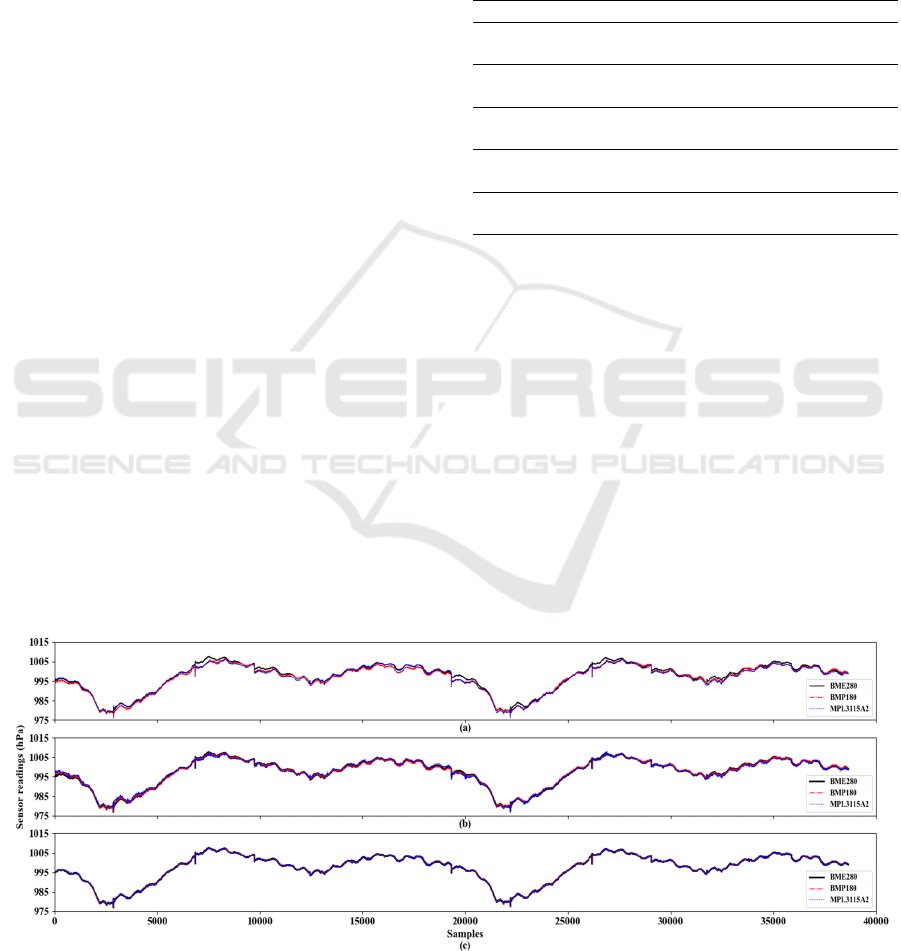
Figure 4 shows the timeseries plots containing

raw readings, the compensated values using low-cost

sensor datasets and the compensated values using

independent sensor readings. It is possible to observe

that there were no significant deviations in data

adjusted by the model that considered all low-cost

sensor data. The abrupt changes visible in the

timeseries plot was caused by appending subsequent

experimental data when the last value of the previous

experiment was different from the first value of the

subsequent one. As these anomalies occurs once after

every 2000+ samples, it does not cause significant

depreciation in numeric performance and is of no

concern.

On the contrary of the model that used all sensors,

the

adjusted

data

that

used

only

the

independent

Figure 4: Timeseries of atmospheric pressure readings: (a) raw data; (b) data adjusted by the model trained with the

independent sensor data; (c) data adjusted by the model trained with the low-cost weather sensors data.

SENSORNETS 2020 - 9th International Conference on Sensor Networks

sensor readings as input presented deviations that can

be visually detected at some points, suggesting that

the reduced number of input features, even from a

certified sensor, may not reach the same efficacy, for

this purpose, as a set of low-cost sensors co-located.

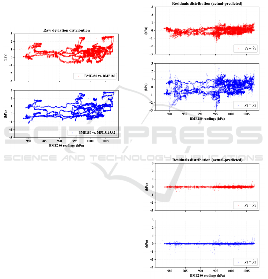
The plot containing the error scattering between

raw vectors is presented in Figure 5, and the residuals

plot (difference between predicted and actual

deviations) of the model trained with the independent

sensor and the model trained with all sensor data are

presented in Figures 6 and 7, respectively.

Figure 5: Deviation distribution of the atmospheric pressure

sensor readings as obtained (raw).

The density of the error scattering can be

interpreted by the colour intensity: faint colours

corresponds to low concentration of deviations; vivid

and solid colours corresponds to higher concentration

of deviations.

An ideal behaviour of the residuals distribution in

a fitted model would be a straight horizontal line on

zero hPa. The residuals plot of the model trained with

the independent sensor (“IS_FIT”) indicates that

there was still a random behaviour of the deviations.

However, it achieved a better performance for

BMP180 than for MPL3115A2, as shown by

comparing Figures 5 and 6.

The residuals scatterplot of the model trained with

all co-located low-cost sensor data (“LC_FIT”)

presents a very low spread around zero: a good

approximation to the ideal behaviour for a fitted

model.

The positive results obtained by the Extremely

Random Trees algorithm, when using readings from

all co-located low-cost sensors, can be extended to the

correction of outliers. Although it is still possible to

perceive the presence of few outliers in Figure 7 (the

vertically spaced points around 983hPa and 995hPa),

they were significantly reduced if compared to the

“IS_FIT” model residuals. Based on these

observations, it can be concluded that the “LC_FIT”

managed to notoriously reduce the readings

deviations.

Figure 6: Residuals distribution of Extremely Random

Trees ensemble regressor trained with temperature,

humidity and dew point estimative from independent sensor

(“IS_FIT”).

Figure 7: Residuals distribution of Extremely Random

Trees ensemble regressor trained with temperature and

humidity from co-located low-cost sensors (“LC_FIT”).

The determination coefficients (r²) and

Spearman’s rank-order correlation coefficient (ρ) of

Deviation Prediction and Correction on Low-Cost Atmospheric Pressure Sensors using a Machine-Learning Algorithm

the datasets, before and after the Extremely Random

Tree algorithm fitting, are exposed in Table 2. The

lowest r² was observed between BME280 and

MPL3115A2 in raw datasets, with a value of 0.9798;

the highest r² was observed in “LC_FIT” datasets,

with both vectors exceeding the 0.9999 value when

compared to BME280. The lowest ρ was also

observed between BME280 and MPL3115A2 in raw

datasets, with a value of 0.9861, and the highest ρ was

also observed in “LC_FIT” datasets, with both

vectors exceeding the value of 0.9999.

Table 2: Determination coefficients (r²) and Spearman’s

rank-order correlation coefficient (ρ) between atmospheric

pressure sensor readings before and after deviation

compensation by the machine-learning model.

Dataset

BME280 versus:

BMP180 MPL3115A2

“Raw”

r² 0.9815 0.9798

ρ 0.9909 0.9861

“IS_FIT”

r² 0.9982 0.9905

ρ 0.9982 0.9913

“LC_FIT”

r² 0.9999+ 0.9999+

ρ 0.9999+ 0.9999+

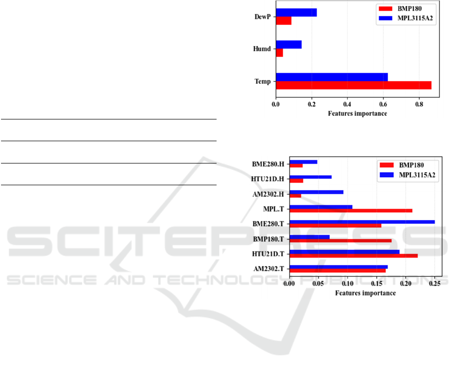
To enrich the interpretation on how the model

managed to predict the errors, it is relevant to analyse

the feature importance plot. This information can be

obtained from the Extremely Randomized Forest

model. It reveals which features had an informative

role during the training of the model and which

features do not inflict significative influence in the

outputs. In other words, and for this case, it permits

the determination of which data the error of evaluated

atmospheric pressure sensors depends on. The feature

importance plot for the model trained with the

independent sensor (“IS_FIT”) is presented in Figure

8, whilst the feature importance plot of low-cost

trained model (“LC_FIT”) is presented in Figure 9.

The interpretation of Figure 8 points out that the

BMP180 sensor deviations were mostly temperature

dependent (87% of importance), while the

MPL3115A2 deviations demonstrated to suffer

higher, yet small, influence from relative humidity

(14% of importance, versus 2.5% for BMP180). The

dewpoint, calculated by a non-linear formula that

considers both temperature and humidity, presented

relevant importance for MPL3115 deviation

predictions (above 20% of importance) while it had

no significant impact on BMP180 deviation

predictions.

Regarding the quantities dependence, the model

trained with low-cost sensors (Figure 9) agreed with

the information presented by the model trained with

the independent sensor: the sum of temperature

sensors importance resulted in 93% for the BMP180,

and humidity has no informative role (7%).

Meanwhile, the sum of humidity data importance

results in 20% for MPL3115A2, suggesting that this

variable may be considered for this sensor calibration

Figure 8: Features importance plot of input vectors used for

training the IS_FIT model.

Figure 9: Features importance plot of input vectors used for

training the LC_FIT model.

As achieved results were considered positive, no

additional hyper-parameter tuning was performed in

the machine-learning model. However, it is not

discarded that a fine tuning could enhance the

algorithm’s performance.

6 DISCUSSION AND

CONCLUSIONS

In this paper, the utilization of a set of co-located low-

cost sensors with post-processing in an accessible

machine-learning algorithm showed promising

results for atmospheric pressure sensor error

prediction, once the deviations were reduced by more

than 90% for both sensor models. The achieved

reduction on the observed deviations between the

sensors, and the consequent data quality

SENSORNETS 2020 - 9th International Conference on Sensor Networks

enhancement, through the utilization of machine

learning algorithms is in agreement with the studies

presented by (Yamamoto et al., 2017) and

(Zimmerman et al., 2018), which used machine

learning resources to improve the data quality from

temperature and air quality sensors, respectively.

Despite the model trained with the independent

sensor was able to reduce deviations between the

sensor pairs in acceptable levels, it still did not reach

the same performance as the model that learned the

error behaviour using the entire low-cost sensors

dataset. In a broader reasoning, the low-cost of a

given sensor might imply a trade-off on its data

quality, but the presented results point out that, if a

group of low-cost sensors is used and its data is

handled properly (e.g. synchrony, logging and data

treatment), the deviation prediction process, and its

correction, may be more effective than when just one

certified sensor is used. This observation also

corroborates with one of the main points of the

collaborative sensing that is spreading the low-cost

sensor units (fixed or mobile) to overcome the quality

of a singular sensing node. Then, it may act as a

complementary asset to help conventional methods to

address a problem, or even be a palliative in certain

situations (Giordano & Puccinelli, 2015). An

example that illustrates the low-cost sensors playing

informative role in places where conventional

methods are not available yet in large scale is the

project with low-cost weather stations for developing

countries described by (Mwangi, 2017), that used the

HTU21D and BMP180 sensors – both used in this

paper. The stations were tested in NOAA facilities

and then deployed into field in Kenya for continuous

weather monitoring in remote places. Such work can

expand into an enhanced environmental sensor

network involving the “low-cost” concept, but with

“certified” results, similar to the work presented by

(Ingelrest et al., 2010).

Regarding the analysis, the most intuitive

example of potential application from the observed

outcomes is a real time calibration service using a

previously trained machine-learning model.

Although the model was trained with offline data,

after the learning process, it can be executed online,

in real time. This is possible to be done by performing

the object serialization (or model persistence) in

Python programming language, for example. In short,

it allows the serialization (export) of an offline trained

object (e.g. the trained Extremely Random Trees

ensemble regressor used in this work) into a stream of

bytes and performs its portability (import) to other

service, such as an online server, or a middleware,

similar to the author’s proposals about data quality

improvements in (Dua et al., 2009; Fersi, 2015).

It should be highlighted that the presented results

were obtained by considering the BME280 as a

beacon (a non-certified reference). However, these

results do not show any evidence that they could not

be replicated and reach similar positive performance

if the target vectors (



and



) were obtained from a

reference sensor for atmospheric pressure instead of

a beacon sensor, since the machine learning is able to

predict the error behaviour regardless of the number

of inputs. Although the environmental dependence of

the error between atmospheric pressure sensor were

expected, since the considered physical quantities are

strictly related one to another, the Extra-Trees

algorithm would manage to pick only the features that

relevantly can describe the observed problem. In

other words, if the input had more, and even

irrelevant, features (e.g. timestamp, luminosity, etc),

the obtained results would not be different.

From this point on, some possibilities of

subsequent works can be considered, such as: a field

test (uncontrolled conditions) of the error prediction

using the approach of this work, and the consequent

evaluation of its robustness for long-term sensor use,

or its robustness over sensor positioning (spatial

variation); the investigation of the performance of this

approach when using a certified reference sensor for

atmospheric pressure as the generator for the target

vectors (instead of a beacon sensor, as

aforementioned); to assess the performance of

different machine learning algorithms for offline and

online sensor correction (e.g. Random Forests, SVM

regressor, Lasso, etc.) and different hyper parameters

tuning.

Finally, it is expected that the presented work, its

respective results, and the opened opportunities may

provide contributions or further motivations for

studies situated in the intersection zone between

citizen science, big data and environmental awareness

and monitoring, or even those beyond these areas but

which objectives eventually include the enhancement

of data quality from environmental microsensors.

REFERENCES

Adafruit. (2016). AM2302/DHT22 Datasheet (pp. 1–5). pp.

1–5. Retrieved from https://cdn-

shop.adafruit.com/datasheets/Digital+humidity+and+t

emperature+sensor+AM2302.pdf

Allen, J. G., MacNaughton, P., Satish, U., Santanam, S.,

Vallarino, J., & Spengler, J. D. (2016). Associations of

cognitive function scores with carbon dioxide,

ventilation, and volatile organic compound exposures

Deviation Prediction and Correction on Low-Cost Atmospheric Pressure Sensors using a Machine-Learning Algorithm

in office workers: A controlled exposure study of green

and conventional office environments. Environmental

Health Perspectives, 124(6), 805–812.

https://doi.org/10.1289/ehp.1510037

Ashcroft, M. B. (2018). Which is more biased:

Standardized weather stations or microclimatic

sensors? Ecology and Evolution, 5231–5232.

https://doi.org/10.1002/ece3.3965

Borrego, C., Costa, A. M., Ginja, J., Amorim, M.,

Coutinho, M., Karatzas, K., … Penza, M. (2016).

Assessment of air quality microsensors versus

reference methods: The EuNetAir joint exercise.

Atmospheric Environment, 147(2), 246–263.

https://doi.org/10.1016/j.atmosenv.2016.09.050

Bosch Sensortec. (2013). BMP180 Datasheet (p. 28). p. 28.

Retrieved from https://cdn-

shop.adafruit.com/datasheets/BST-BMP180-DS000-

09.pdf

Bosch Sensortec. (2015). BME280 Datasheet. Retrieved

from http://www.bosch-

sensortec.com/en/homepage/products_3/environmenta

l_sensors_1/bme280/bme280_1

Castell, N., Dauge, F. R., Schneider, P., Vogt, M., Lerner,

U., Fishbain, B., … Bartonova, A. (2017). Can

commercial low-cost sensor platforms contribute to air

quality monitoring and exposure estimates?

Environment International, 99, 293–302.

https://doi.org/10.1016/j.envint.2016.12.007

D’Hondt, E., Stevens, M., & Jacobs, A. (2013).

Participatory noise mapping works! An evaluation of

participatory sensing as an alternative to standard

techniques for environmental monitoring. Pervasive

and Mobile Computing, 9(5), 681–694.

https://doi.org/10.1016/j.pmcj.2012.09.002

de Araújo, T. C., Silva, L. T., & Moreira, A. C. (2017). Data

Quality Issues on Environmental Sensing with

Smartphones. Proceedings of the 6th International

Conference on Sensor Networks: SENSORNETS., 59–

68. https://doi.org/10.5220/0006201600590068

Dua, A., Bulusu, N., & Feng, W. (2009). Towards

Trustworthy Participatory Sensing. 4th USENIX

Workshop on Hot Topics in Security (HotSec-09).

Duvall, R., Long, R., Beaver, M., Kronmiller, K., Wheeler,

M., & Szykman, J. (2016). Performance Evaluation and

Community Application of Low-Cost Sensors for

Ozone and Nitrogen Dioxide. Sensors, 16(10), 1698.

https://doi.org/10.3390/s16101698

Fersi, G. (2015). Middleware for internet of things: A study.

Proceedings - IEEE International Conference on

Distributed Computing in Sensor Systems, DCOSS

2015, 2(3), 230–235.

https://doi.org/10.1109/DCOSS.2015.43

Freescale Semiconductor. (2013). MPL3115A2 Datasheet.

Retrieved from https://cdn-

shop.adafruit.com/datasheets/1893_datasheet.pdf

Fuertes, W., Carrera, D., Villacis, C., Toulkeridis, T.,

Galarraga, F., Torres, E., & Aules, H. (2015).

Distributed System as Internet of Things for a New

Low-Cost, Air Pollution Wireless Monitoring on Real

Time. 2015 IEEE/ACM 19th International Symposium

on Distributed Simulation and Real Time Applications

(DS-RT), 58–67. https://doi.org/10.1109/DS-

RT.2015.28

Geurts, P., Ernst, D., & Wehenkel, L. (2006). Extremely

randomized trees. Machine Learning, 63(1), 3–42.

https://doi.org/10.1007/s10994-006-6226-1

Giordano, S., & Puccinelli, D. (2015). When sensing goes

pervasive. Pervasive and Mobile Computing, 17(PB),

175–183. https://doi.org/10.1016/j.pmcj.2014.09.008

Gitzel, R. (2016). Data quality in time series data: An

experience report. CEUR Workshop Proceedings,

1753, 41–49.

Goldman, J., Shilton, K., Burke, J., Estrin, D., Hansen, M.,

Ramanathan, N., … Samanta, V. (2009). Participatory

Sensing - A Citizen-powered approach to illuminating

the patterns that shape our world. Los Angeles,

California, USA: Center for Embedded Networked

Sensing.

Hu, K., Sivaraman, V., Luxan, B. G., & Rahman, A. (2016).

Design and Evaluation of a Metropolitan Air Pollution

Sensing System. IEEE Sensors Journal, 16(5), 1448–

1459.

Ingelrest, F., Barrenetxea, G., Schaefer, G., Vetterli, M.,

Couach, O., & Parlange, M. (2010). Sensorscope:

Application-Specific Sensor Network for

Environmental Monitoring. ACM Transactions on

Sensor Networks, 6(2), 1–32.

https://doi.org/10.1145/1689239.1689247

Kanhere, S. S. (2011). Participatory Sensing:

Crowdsourcing Data from Mobile Smartphones in

Urban Spaces. 2011 IEEE 12th International

Conference on Mobile Data Management, 3–6.

https://doi.org/10.1109/MDM.2011.16

Kumar, P., Morawska, L., Martani, C., Biskos, G.,

Neophytou, M., Di Sabatino, S., … Britter, R. (2015).

The Rise of Low-Cost Sensing for Managing Air

Pollution in Cities. Environment International, 75,

199–205. https://doi.org/10.1016/j.envint.2014.11.019

Lascar Electronics. (n.d.). Certificate of Calibration.

Retrieved June 28, 2016, from

http://www.lascarelectronics.com/pdf-usb-

datalogging/data-logger0800188001331301358.pdf

Liu, L., Wei, W., Zhao, D., & Ma, H. (2015). Urban

Resolution: New Metric for Measuring the Quality of

Urban Sensing. IEEE Transactions on Mobile

Computing, 14(12), 2560–2575.

https://doi.org/10.1109/TMC.2015.2404786

Magli, S. ., Lodi, C. ., Contini, F. M. ., Muscio, A. ., &

Tartarini, P. . (2016). Dynamic analysis of the heat

released by tertiary buildings and the effects of urban

heat island mitigation strategies. Energy and Buildings,

114, 164–172.

https://doi.org/10.1016/j.enbuild.2015.05.037

Measurement Specialties Inc. (2013). HTU21D Datasheet

(pp. 1–21). pp. 1–21. Retrieved from https://cdn-

shop.adafruit.com/datasheets/1899_HTU21D.pdf

Minh-Dung, N., Takahashi, H., Uchiyama, T., Matsumoto,

K., & Shimoyama, I. (2013). A barometric pressure

sensor based on the air-gap scale effect in a cantilever.

SENSORNETS 2020 - 9th International Conference on Sensor Networks

Applied Physics Letters, 103(14), 103–106.

https://doi.org/10.1063/1.4824027

Mwangi, C. (2017). Low Cost Weather Stations for

Developing Countries (Kenya). 7th United Nations

International Conference on Space-Based

Technologies for Disaster Risk Reduction, (October).

Retrieved from http://www.un-

spider.org/sites/default/files/21. UNSPIDER

Presentation - Mwangi.pdf

Özgür, E., & Koçak, K. (2015). The effects of the

atmospheric pressure on evaporation. Acta

Geobalcanica, 1(1), 17–24.

https://doi.org/10.18509/agb.2015.02

Piedrahita, R., Xiang, Y., Masson, N., Ortega, J., Collier,

A., Jiang, Y., … Shang, L. (2014). The next generation

of low-cost personal air quality sensors for quantitative

exposure monitoring. Atmospheric Measurement

Techniques, 7(10), 3325–3336.

https://doi.org/10.5194/amt-7-3325-2014

Qaid, A., Bin Lamit, H., Ossen, D. R., & Raja Shahminan,

R. N. (2016). Urban heat island and thermal comfort

conditions at micro-climate scale in a tropical planned

city. Energy and Buildings, 133, 577–595.

https://doi.org/10.1016/j.enbuild.2016.10.006

Saini, H., Thakur, A., Ahuja, S., Sabharwal, N., & Kumar,

N. (2016). Arduino based automatic wireless weather

station with remote graphical application and alerts. 3rd

International Conference on Signal Processing and

Integrated Networks, SPIN 2016, 605–609.

https://doi.org/10.1109/SPIN.2016.7566768

Salata, F., Golasi, I., Petitti, D., Vollaro, E. de L., Coppi,

M., & Vollaro, A. de L. (2017). Relating microclimate,

human thermal comfort and health during heat waves:

an analysis of heat island mitigation strategies through

a case study in an urban outdoor environment.

Sustainable Cities and Society, 30, 79–96.

https://doi.org/10.1016/j.scs.2017.01.006

Satish, U., Mendell, M. J., Shekhar, K., Hotchi, T.,

Sullivan, D., Streufert, S., & Fisk, W. J. (2012). Is CO2

an indoor pollutant? direct effects of low-to-moderate

CO2 concentrations on human decision-making

performance. Environmental Health Perspectives,

120(12), 1671–1677.

https://doi.org/10.1289/ehp.1104789

Scikit-Learn. (2019). Scikit-Learn. Retrieved from

https://scikit-learn.org/stable/

Silva, L. T., & Mendes, J. F. G. (2012). City Noise-Air: An

environmental quality index for cities. Sustainable

Cities and Society, 4(1), 1–11.

https://doi.org/10.1016/j.scs.2012.03.001

Sinha, N., Pujitha, K. E., & Alex, J. S. R. (2015). Xively

based sensing and monitoring system for IoT. 2015

International Conference on Computer Communication

and Informatics, ICCCI 2015, 8–13.

https://doi.org/10.1109/ICCCI.2015.7218144

Sivaraman, V., Carrapetta, J., Hu, K., & Luxan, B. G.

(2013). HazeWatch: A participatory sensor system for

monitoring air pollution in Sydney. 38th Annual IEEE

Conference on Local Computer Networks - Workshops,

56–64. https://doi.org/10.1109/LCNW.2013.6758498

Szczurek, A., Maciejewska, M., & Pietrucha, T. (2017).

Occupancy detection using gas sensors. SENSORNETS

2017 - Proceedings of the 6th International Conference

on Sensor Networks, 2017-Janua(Sensornets), 99–107.

Terando, A. J., Youngsteadt, E., Meineke, E. K., & Prado,

S. G. (2017). Ad hoc instrumentation methods in

ecological studies produce highly biased temperature

measurements. Ecology and Evolution, 7(23), 9890–

9904. https://doi.org/10.1002/ece3.3499

Trilles, S., Luján, A., Belmonte, Ó., Montoliu, R., Torres-

Sospedra, J., & Huerta, J. (2015). SEnviro: A

sensorized platform proposal using open hardware and

open standards. Sensors (Switzerland), 15(3), 5555–

5582. https://doi.org/10.3390/s150305555

US-EPA. (2019). US EPA. Retrieved from

https://www.epa.gov/environmental-topics/air-topics

Yamamoto, K., Togami, T., Yamaguchi, N., & Ninomiya,

S. (2017). Machine learning-based calibration of low-

cost air temperature sensors using environmental data.

Sensors (Switzerland), 17(6), 1–16.

https://doi.org/10.3390/s17061290

Young, D. T., Chapman, L., Muller, C. L., Cai, X.-M., &

Grimmond, C. S. B. (2014). A Low-Cost Wireless

Temperature Sensor: Evaluation for Use in

Environmental Monitoring Applications. Journal of

Atmospheric and Oceanic Technology, 31(4),

140320111908003. https://doi.org/10.1175/JTECH-D-

13-00217.1

Yunus, N., Halin, I., Sulaiman, N., Ismail, N., & Ong, K.

(2015). Valuation on MEMS pressure sensors and

device applications. International Journal of Electrical,

Computer, Energetic, Electronic and Communication

Engineering, 9(8), 768–776.

Zaman, J., D’Hondt, E., Boix, E. G., Philips, E., Kambona,

K., & De Meuter, W. (2014). Citizen-friendly

participatory campaign support. 2014 IEEE

International Conference on Pervasive Computing and

Communication Workshops (PERCOM

WORKSHOPS), 232–235.

https://doi.org/10.1109/PerComW.2014.6815208

Zimmerman, N., Presto, A. A., Kumar, S. P. N., Gu, J.,

Hauryliuk, A., Robinson, E. S., … Subramanian, R.

(2018). A machine learning calibration model using

random forests to improve sensor performance for

lower-cost air quality monitoring. Atmospheric

Measurement Techniques, 11(1), 291–313.

https://doi.org/10.5194/amt-11-291-2018

APPENDIX

The datasets used in this work are available in the

Zenodo repository, with digital identifier (DOI) as

10.5281/zenodo.3560299.

We encourage the readers to reproduce our

findings.

Deviation Prediction and Correction on Low-Cost Atmospheric Pressure Sensors using a Machine-Learning Algorithm