Visual Analysis of Billiard Dynamics Simulation Ensembles

Stefan Boshe-Plois

, Quynh Quang Ngo

, Peter Albers

and Lars Linsen

Westf

alische Wilhelms-Universit

at M

unster, Germany

University of Heidelberg, Germany

Keywords:

Ensemble Visualization, Billiard Dynamics.

Abstract:

Mathematical billiards assume a table of a certain shape and dynamical rules for handling collisions. Some

trajectories exhibit distinguished patterns. Detecting such trajectories manually for a given billiard is cum-

bersome, especially, when assuming an ensemble of billiards with different parameter settings. We propose

a visual analysis approach for simulation ensembles of billiard dynamics based on phase-space visualizations

and multi-dimensional scaling. We apply our methods to the well-studied approach of dynamical billiards for

validation and to the novel approach of symplectic billiards for new observations.

1 INTRODUCTION

In the theory of mathematical dynamical systems the

main question is to investigate the long-term quali-

tative behavior of a system in terms of certain qual-

itative facets. Usually, these facets are phenomena

like periodicity and recurring patterns. Further, it

can be examined whether a system shows stable or

chaotic behavior and how robust it is to perturbations.

Mathematical billiards form a category of dynamical

systems (Birkhoff, 1927). They arise naturally from

physical laws of reﬂection and show connections to

problems like the motion of gas particles in a closed

environment. While the ultimate goal is to give an-

swers based on theoretical proofs, it is useful to have

well-founded suppositions indicating the direction to

head. We present visual analysis methods for sim-

ulation ensembles of billiard dynamics to form such

suppositions.

Billiards are deﬁned on a table and the dynamics

are dependent on the shape of the table (Tabachnikov,

2005). If its boundary is deﬁned via a function, a per-

turbation corresponds to slightly changing a param-

eter in the function. The question is what changes

occur due to such a perturbation, i.e., whether the bil-

liard trajectories exhibit a qualitatively different be-

havior. Since it is a priori unclear, which trajectories

would exhibit changing patterns and at what pertur-

bation levels, we propose to consider a simulation en-

semble with different shape parameters of the table,

compute a large amount of trajectories for each en-

semble member, and use visual analysis methods to

explore the generated data.

To analyze the trajectories of a single ensemble

member, we propose to visualize them in a phase

space spanned by the positions of collisions along

the boundary and directions. To analyze the changes

when altering the table’s parameters we compute pair-

wise dissimilarities between corresponding trajecto-

ries of ensemble members. These dissimilarities can

be visually encoded using a multidimensional scaling

(MDS) approach, which allows for the analysis of the

impact of the different table parameters on the dynam-

ics. Having identiﬁed interesting ensemble member

pairs from the MDS, we support a comparative visu-

alization of that pair by highlighting the deviations in

the trajectories.

While dynamical billiards (Birkhoff, 1927) have

been investigated in great depth, it has not yet been

addressed in detail whether other dynamics such as

symplectic billiards (Albers and Tabachnikov, 2018)

exhibit similar phenomena. We apply our approach

to dynamical billiards to validate our approach and to

symplectric billiards for novel ﬁndings.

2 RELATED WORK

In the visualization community, there have been many

attempts in trying to visually analyze dynamics. Tric-

oche et al. (Tricoche et al., 2012) study conserva-

tive dynamical systems using area-preserving maps.

They apply their method to two example dynamics to

reveal salient structure in the spatial domain. Boe-

ing et al. (Boeing, 2016) investigated chaos and self-

Boshe-Plois, S., Ngo, Q., Albers, P. and Linsen, L.

Visual Analysis of Billiard Dynamics Simulation Ensembles.

DOI: 10.5220/0008956201850192

In Proceedings of the 15th International Joint Conference on Computer Vision, Imaging and Computer Graphics Theory and Applications (VISIGRAPP 2020) - Volume 3: IVAPP, pages

185-192

ISBN: 978-989-758-402-2; ISSN: 2184-4321

185

(a) standard dynamics (b) symplectic dynamics

Figure 1: Billiard dynamics.

similarity in non-linear systems. Ngo et al. (Ngo

et al., 2016) investigated dynamics on networks,

where they compute similarities between the dynam-

ics of the networks’ nodes, which are then visualized

using a multi-dimensional scaling (MDS) approach.

We also make use of MDS to visualize our data, but

apply it to compare simulation runs within an en-

semble of simulations. Kumpf et al. (Kumpf et al.,

2019) investigated ensembles to performed a sensibil-

ity analysis for weather forecasts based on correlation

measures. There aim was to identify regions of robust

prediction, which is related to parts of our goals. Fur-

ther approaches for dynamical systems exist in other

application scenarios. To our knowledge, this is the

ﬁrst paper that investigates how visualization can sup-

port the analysis of billiard dynamics.

3 BACKGROUND AND

REQUIREMENT ANALYSIS

We ﬁrst want to provide the mathematical background

for our investigations. A billiard model consists of a

table and dynamics. A billiard table is a convex do-

main Γ ⊂ R

with a smooth boundary γ := ∂Γ. Of

great interests are, in particular, elliptic billiard ta-

bles deﬁned via a function F : R

→ R with F(x,y) =

−1, a,b > 0, and r, w ≥ 2. The elliptic billiard

table’s boundary is given by γ =

{

(x,y) | F(x,y) = 0

}

Γ is called a standard elliptic table, if r = w = 2, oth-

erwise a perturbed elliptic table.

The billiard dynamics consist of a rule set or algo-

rithm that determines a sequence of collision points

)

n∈N

with A

∈ γ, which we call billiard trajec-

tory. One may simply imagine a massless billiard ball

that moves with unit speed and without friction. The

most natural kind of billiard dynamics are the dynam-

ical or Birkhoff billiards, as they arise from the laws

of elastic collision in physics. Therefore, we also re-

fer to them as standard dynamics. Assume we have

a collision point A on the boundary γ together with a

direction vector v

∈ R

. Then, from a point A with

direction v

, the subsequent point B is obtained as the

intersection of the line A + r · v

, r ∈ R with γ and

the subsequent direction is determined via the reﬂec-

tion law, i.e., the angle of incidence is the same as the

angle of reﬂection, see Figure 1(a).

The standard dynamics can be described as a vari-

ational problem: If A,B,C ∈ γ is a sequence of col-

lisions and we ﬁx A and C, then the position of B

is deﬁned by the condition that |AB| + |BC| is ex-

tremal. In symplectic billiards the dynamics are de-

rived from a related variational problem by the condi-

tion that the area of the triangle ABC is extremal (Al-

bers and Tabachnikov, 2018). The name symplectic

arises from the fact that the map describing the dy-

namics has the standard symplectic form ω as a gen-

erating function. Further mathematical details on the

form ω are beyond the scope of this paper. It suf-

ﬁces to report that the resulting rules for the dynam-

ics can be reduced to taking the position of B to be

such that the vector C − A lies in the tangent space

γ. For computing trajectories on elliptical tables,

we start with two points A and B, compute the tan-

gent v

∈ T

γ, and calculate the root of the function

F(A + r · v

), see Figure 1(b) (Albers and Tabach-

nikov, 2018).

While structures in dynamical billiards have al-

ready been analyzed in much detail, advances for

symplectic billiards are recent. Initial questions that

are to be answered and respective expectations were

formulated by the domain scientists as follows:

• On a standard elliptic table, one would expect

clear structures that should be qualitatively inde-

pendent of parameters a and b for both dynamical

and symplectic billiards.

IVAPP 2020 - 11th International Conference on Information Visualization Theory and Applications

186

(a) standard dynamics (b) standard dynamics (c) standard dynamics

(d) symplectic dynamics (e) symplectic dynamics (f) symplectic dynamics

Figure 2: Trajectories with different starting conditions using boundary function F(x,y) = x

/4 + y

/6 − 1.

• On a perturbed elliptic table, there should occur

small anomalies (i.e., trajectories change in quali-

tative aspects) for dynamical billiards, but it is an

open question, whether the same is true for sym-

plectic billiards.

• If some trajectories change qualitatively when

perturbing the elliptic table, one would like to

know how they look like.

• It is unclear what happens, if one changes the pa-

rameters a and b on a perturbed elliptic table. It

would be interesting to see, whether there exist re-

lations between the two parameters depending on

their ratio.

To answer these questions, we generate and visu-

ally analyze simulation ensembles for both dynamical

and symplectic billiards by varying parameters r and

w as well as parameters a and b. For each ensemble

member, we compute a large amount of trajectories

with different starting collisions and directions for a

sufﬁciently large number of collisions.

From the expectations and questions formulated

by the domain scientists, we extracted the require-

ments to our analysis system as follows:

1. The highest-level goal is understand the inﬂuence

of the parameter settings on the dynamics. Hence,

we need to analyze the entire ensemble simulta-

neously.

2. When two ensemble runs differ, it would be of

interest to see, which of their trajectories differ.

Hence, we need a comparative visualization of

trajectories of two runs.

3. On the lowest level, one is interested in observing

individual simulation runs and observe the behav-

ior of their trajectories.

4 VISUAL ANALYSIS

In this section, we describe the visualization meth-

ods we developed for analyzing individual ensemble

members, ensemble member pairs, and entire ensem-

bles.

4.1 Phase-space Visualization

Our ﬁrst aim is to visualize trajectories of a single

ensemble member (cf. Requirement 3). A straight-

forward visual encoding of a simulation outcome is

to render the trajectories on the table. Figure 2 shows

respective examples for standard and symplectic bil-

liards. The visualizations clearly exhibit patterns, but

only for a single trajectory. Obviously, displaying

many such trajectories simultaneously leads to visual

clutter. Therefore, we propose to visualize the set of

trajectories for a single ensemble member in a phase-

space conﬁguration.

A phase space Ω for dynamical billiards consists

of a collision point on the boundary together with a

direction vector, i.e., Ω = γ × R

. Equivalently, it

Visual Analysis of Billiard Dynamics Simulation Ensembles

187

(a) Ω = S

× [0,π) (b) Ω = S

× [0,π)

× S

(d) Ω = S

× S

Figure 3: Phase-space visualizations of sets of trajectories (with random color mapping) using boundary function F(x, y) =

/4 + y

/6 − 1 for standard (a,b) and symplectic dynamics (c,d).

can be deﬁned by describing the direction using the

angle to the tangent at the collision point, i.e., Ω =

γ × [0,π]. Furthermore, one can apply a parametriza-

tion to the curve γ. Since γ is closed, we denote such

a parametrization as α : S

→ γ, which is equivalent

to α : [s,t] → γ with α(s) = α(t). The phase space

then becomes Ω = S

× [0, π] or Ω = [s,t] × [0,π].

For elliptical tables, we chose the parametrization

α(p) = arccos (hp − q

i) with a center point q

∈ Γ

and a reference vector v

∈ S

. We used q

= (0, 0)

and v

= (1, 0). For symplectic billiards, a conﬁgu-

ration is not deﬁned by a collision point and a direc-

tion vector, but by two consecutive collision points.

Hence, we deﬁne the phase space by Ω = S

× S

Ω = [s,t] × [s,t], respectively.

Having deﬁned a phase space, a single trajectory

can be visualized by plotting the respective collisions

as dots in the phase space. A set of trajectories of

a single ensemble member can, then, be shown by

coloring each trajectory with a unique color. For

the color mapping we considered categorical color

maps, but given the large amount of trajectories, there

are not enough colors that can be sufﬁciently well

distinguished. Thus, random color mapping worked

equally well, i.e., each trajectory just got a randomly

assigned color. Figure 3 shows respective examples

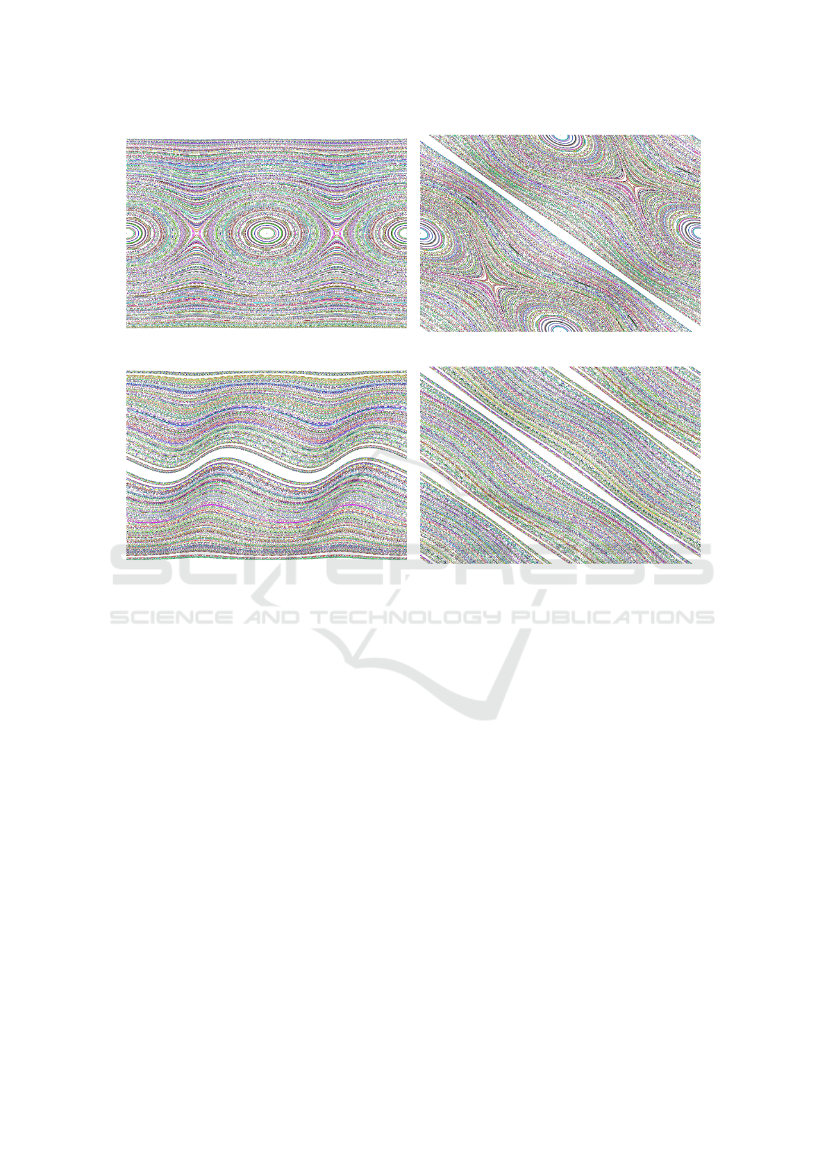
for standard and symplectic billiards.

4.2 Comparative Visualization

Our Requirement 2 was to visually compare two en-

semble members to observe where and how trajecto-

ries differ, e.g., to highlight anomalies. From the jux-

taposed phase-space visualizations in Figure 4(a,b),

we can conclude that it is difﬁcult to detect small

differences. Hence, the design choice would be to

compute an explicit visual encoding of computed dif-

ferences. To highlight the differences, we have to

compute the differences between two ensemble mem-

bers. More precisely, we have to compute the dif-

ferences of corresponding trajectories in the two en-

semble members. Using the phase-space representa-

tion of starting conﬁgurations for trajectory compu-

tations, we can generate matching starting conditions

for each ensemble member. Hence, when comparing

two ensemble members, we have a set of pairs of cor-

IVAPP 2020 - 11th International Conference on Information Visualization Theory and Applications

188

(a) standard elliptic table (b) perturbed elliptic table

Figure 4: Juxtaposed visualization of two simulation runs using standard dynamics with parameters (a) a = 7,b = 4,r = 2, w =

2 and (b) a = 7,b = 4, r = 2.001,w = 2. (c) The comparative visualization highlights differences based on color mapping the

trajectories’ distances d

. (d) When perturbing the standard elliptic table (a = 4, b = 6, r = w = 2) by increasing parameters

r = 2.001 and w = 2.005, the comparative visualization for symplectic dynamics highlights qualitative changes in the form of

cyclic structures.

responding trajectories.

Let A = (A

)

1≤ j≤n

and B = (B

)

1≤ j≤n

be a pair of

corresponding trajectories. We deﬁne the difference

of two collision points using a Euclidean metric by

) =



j,1

− B

j,1

+ |A

j,2

− B

j,2



with |x − y|

= min(|x − y|,l − |x − y|) being the dis-

tance of two points in an interval quotient space with

length l homeomorphic to S

. The difference of the

trajectories is, then, deﬁned as the average difference

of the collision points, i.e.,

(A,B) =

∑

j=1

)

Having computed the distances d

(A,B) for all tra-

jectory pairs, we can highlight those trajectories A (or

B respectively), where the differences are strongest.

We achieve this by a applying a color mapping to the

trajectories that maps the distances (after normaliza-

tion to the unit interval) linearly from a background

color to a foreground color. Thus, the more different

trajectory A is from trajectory B the more it is empha-

sized. Figure 4(c) shows such a comparative visual-

ization of two ensemble members.

4.3 Ensemble Visualization

Our ﬁnal aim is to fulﬁll Requirement 1, i.e., to al-

low for an analysis of an entire ensemble to investi-

gate the impact of the simulation parameters. Thus,

we need to compare ensemble members at a global

scale. Let S

and S

be two simulation runs each con-

taining m trajectories A

(i)

1≤i≤m

and B

(i)

1≤i≤m

. Building

upon the distance metric d

(i)

) for correspond-

ing trajectory pairs, we deﬁne the difference between

two simulation runs by the average of the distances of

all corresponding trajectory pairs, i.e., we deﬁne

) =

∑

i=1

(i)

)

We compute this distance for each pair of simulation

runs in a given ensemble. The pairwise distances for

Visual Analysis of Billiard Dynamics Simulation Ensembles

189

(a) inﬂuence of ratio a/b (b) inﬂuence of parameter r

Figure 5: Color coding the MDS plots by parameter values for symplectic billiards ensemble shows that r and w are the key

parameters.

an ensemble of k simulation runs can be stored in a

symmetric k × k distance matrix

D = (d

))

1≤i, j≤k

The ensemble visualization shall depict the sim-

ilarities (or distances) of all ensemble members.

Hence, we want to ﬁnd a 2D embedding, where the

2D Euclidean distances of the points that represent

the ensemble members in the embedding resemble the

distances stored in distance matrix D. This is exactly

the objective of the classical metric multi-dimensional

scaling (MDS) approach. Of course, plenty of other

embeddings exist in literature, but MDS reﬂects our

goal of preserving the computed distances by mini-

mizing the stress function (Kruskal and Wish, 1978).

For the implementation, we follow the standard so-

lution via an eigendecomposition of the Gram ma-

trix (Jung, ).

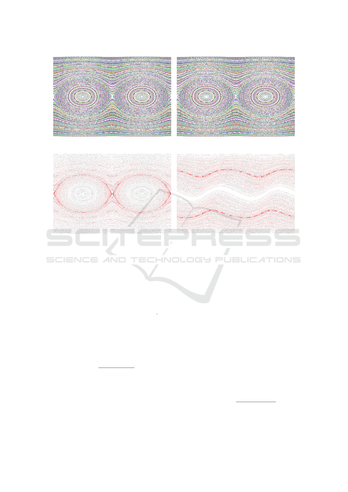
The outcome of the MDS step is visualized in the

form of a 2D scatterplot. Since our goal is to de-

tect the inﬂuence of the billiard table’s parameter, we

support color mapping of the scatterplot with respect

to interactively selected parameters or their ratio, see

Figure 5.

5 RESULTS AND DISCUSSION

We apply our methods to simulation ensembles for

standard and symplectic billiard dynamics to answer

the questions raised in Section 3. We ﬁrst investigated

the impact of the choice of parameters a and b by con-

sidering a circular table (a = b = 1, r = w = 2) and

perturbing it slightly (a = 1.002). For standard dy-

namics, the phase-space visualizations on a circular

table exhibits straight trajectories, as the angles are

not changing, see Figure 6(a). However, when alter-

ing parameter a slightly, the behavior changes qualita-

tively, as trajectories with periodic orbits emerge, see

Figure 6(b). This ﬁnding conﬁrms what was expected

and known from literature. Surprisingly though, this

IVAPP 2020 - 11th International Conference on Information Visualization Theory and Applications

190

(a) a = 1 (b) a = 1.002

Figure 6: Phase-space visualizations of standard dynamics on circular (a) and slightly perturbed circular table (b) show the

emergence of qualitatively different trajectories when changing parameter a.

was not true for symplectic dynamics, where phase-

space visualization for the perturbed table remained

qualitatively equivalent to Figure 6(a). When increas-

ing the ellipticity of the table (e.g., further increas-

ing parameter a), the phase-space visualizations for

standard dynamics exhibit more and more orbit struc-

tures, see Figure 3(a), while phase-space visualization

for symplectic dynamics still consists of horizontal

curves but with waves of increasing amplitudes, see

Figure 3(b).

As a second investigation, we looked into the im-

pact of the choice of parameters r and w by comparing

a standard elliptic table to a perturbed one. For stan-

dard dynamics, the phase-space visualizations seem

almost identical when slightly increasing r from 2 to

2.001, see Figure 4(a,b), but the comparative visu-

alization exhibits some structural changes, see Fig-

ure 4(c). In this investigation, the same holds true for

symplectic dynamics: The comparative visualization

in Figure 4(d) highlights emerging cyclic structures

for perturbed tables, which have not been observed

for the standard elliptic table (cf. Figure 3(b)).

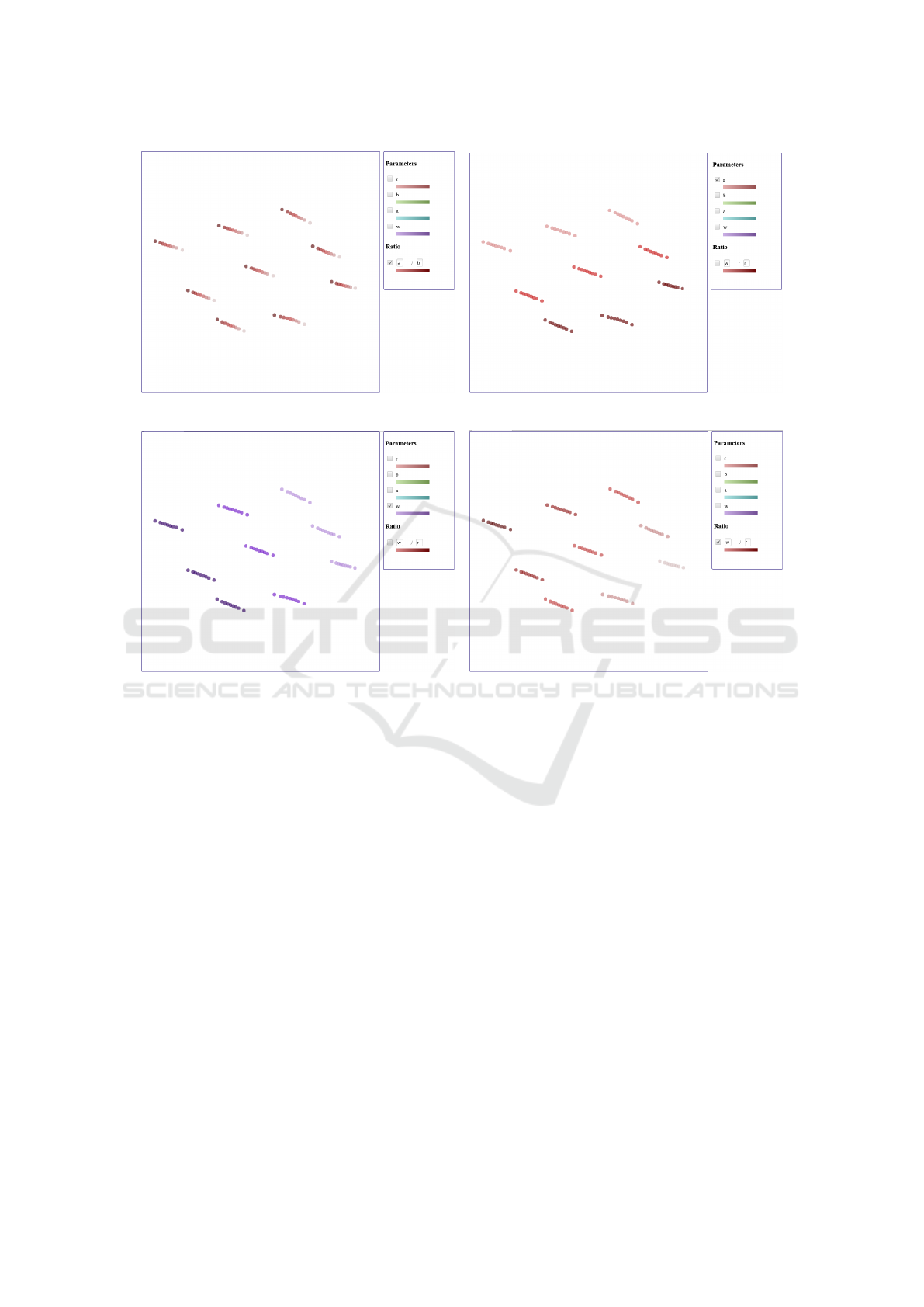
Based on these initial investigation, we generated

ensembles with many different parameter conﬁgura-

tions. For standard dynamics, we generated initial

collisions by sampling the phase space equidistantly

with 23 position × 31 direction samples. For each

initial collision, we computed a trajectory with 200

collision points. These 23 × 31 trajectories are com-

puted for each ensemble member, where the ensem-

ble is formed by choosing parameters from ranges

a ∈ [4;4.004], b ∈ [5; 5.001], r = 2, and w ∈ [2; 2.009]

with step size 0.001. The MDS plot exhibits an arc

shape, see Figure 7. Color coding the plot to inves-

tigate the impact of the parameter, we can make the

following observations: The color transitions for pa-

rameters a, b, or their ratio a/b conﬁrm the observa-

tion from above that these parameters locally affect

the outcome, see Figure 7(b,c). The color transitions

in Figure 7(b,c) form clusters, i.e., we see groups of

points where colors go from dark to bright and then

this pattern is repeated for the next group. Investigat-

ing the inﬂuence of parameter w in Figure 7(a) pro-

vides a different picture: There is a trend of having

brighter colors to the left of the arc and darker colors

to the right, but the transition is not monotonic. How-

ever, when investigating the color transition for ratio

r/w in Figure 7(d), we observe that there is a mono-

tonic color transition from bright to dark that clearly

follows the arc. Hence, we can formulate the suppo-

sition that ratio r/w is the dominant factor for signif-

icant changes, as runs occur the more similar in the

MDS plot the more they have a similar ratio. This is

in accordance with earlier studies in the ﬁeld.

Finally, we generate a simulation ensemble for

symplectic dynamics using the same initial collisions

and trajectory lengths as above, while choosing pa-

rameters from ranges a ∈ [4; 4.006], b ∈ [6; 6.006],

r ∈ [2; 2.006], and w ∈ [2; 2.006] with step size 0.001.

Here, such studies had not been performed yet, but

is easily supported by our tool. Figure 5 shows that

parameters r and w and their ratio r/w are, again, re-

sponsible for generating main trends and clusters in

the MDS plots, while parameters a, b and their ratio

a/b are only responsible for small variations within

the clusters. Figure 5(a) clearly shows the color tran-

sitions only within each of the nine clusters for the

ratio a/b. For parameter r, there is a transition that

creates three stripes of brightness from the upper left

to the lower right. Similarly, for parameter w, there

is a transition that creates three stripes of brightness

from the lower left to the upper right. When combin-

ing the two parameters by looking at their ratio r/w,

there is a transition from left to right with ﬁve stripes.

Hence, we can conclude that for both standard and

symplectic dynamics changes of ratio r/w dominate

Visual Analysis of Billiard Dynamics Simulation Ensembles

191

(a) inﬂuence of parameter w (b) inﬂuence of ratio a/b

Figure 7: The main structure in the MDS visualization of the standard billiards ensemble is governed by ratio r/w.

over changes of ratio a/b. This is a novel ﬁnding that

had not been reported yet.

6 CONCLUSION

We have presented a novel approach to analyze bil-

liards using ensemble visualizations. For standard dy-

namics, we were able to conﬁrm prior studies, while

for symplectic dynamics we made new discoveries

leading to suppositions that are a good starting point

for theoretical proofs.

REFERENCES

Albers, P. and Tabachnikov, S. (2018). Introducing sym-

plectic billiards. Advances in Mathematics, 333:822 –

867.

Birkhoff, G. (1927). Dynamical Systems. American Mathe-

matical Society / Providence, Estados Unidos. Amer-

ican Mathematical Society.

Boeing, G. (2016). Visual analysis of nonlinear dynamical

systems: Chaos, fractals, self-similarity and the limits

of prediction. Systems, 4:37.

Jung, S. Lecture Notes: Multidimensional scaling, Ad-

vanced Applied Multivariate Analysis.

Kruskal, J. and Wish, M. (1978). Multidimensional Scaling.

Number Nr. 11 in 07. SAGE Publications.

Kumpf, A., Rautenhaus, M., Riemer, M., and Westermann,

R. (2019). Visual analysis of the temporal evolution of

ensemble forecast sensitivities. IEEE Transactions on

Visualization and Computer Graphics, 25(1):98–108.

Ngo, Q. Q., H

utt, M.-T., and Linsen, L. (2016). Visual

Analysis of Governing Topological Structures in Ex-

citable Network Dynamics. Computer Graphics Fo-

rum, 35(3):301–310.

Tabachnikov, S. (2005). Geometry and billiards. Stu-

dent Mathematical Library. 30. American Mathemat-

ical Society, Providence, RI; Mathematics Advanced

Study Semesters, University Park, PA,.

Tricoche, X., Garth, C., Sanderson, A., and Joy, K. (2012).

Visualizing Invariant Manifolds in Area-Preserving

Maps, pages 109–124. Springer Berlin Heidelberg,

Berlin, Heidelberg.

IVAPP 2020 - 11th International Conference on Information Visualization Theory and Applications

192