PySpot: A Python based Framework for the Assessment of

Laser-modiﬁed 3D Microstructures for Windows and Raspbian

Hannah Janout

1 a

, Bianca Buchegger

2,3 b

, Andreas Haghofer

1 c

, Dominic Hoeglinger

Jaroslaw Jacak

2 d

, Stephan Winkler

1 e

and Armin Hochreiner

2 f

University of Applied Sciences Upper Austria, School of Informatics, Communications and Media,

Softwarepark 11, 4232 Hagenberg, Austria

University of Applied Sciences Upper Austria, School of Medical Engineering and Applied Social Sciences,

Garnisionstraße 21, 4240 Linz, Austria

Johannes Kepler University Linz, Institute of Applied Physics, Altenberger Straße 69, 4040 Linz, Austria

Keywords:

Image Processing Methods, Fluorescence Microscopy, 3D Microstructures, Image Analysis, Software

Development, Bioinformatics.

Abstract:

Biocompatible 3D microstructures created with laser lithography and modiﬁed for optimal cell growth with

laser grafting, can imitate the 3D structure cells naturally grow in. For the evaluation of the quality and success

of those 3D microstructures, specialized software is required. Our software PySpot can load 2D and 3D images

and analyze those through image segmentation, edge detection, and surface plots. Additionally, the creation

and modiﬁcation of regions of interest (ROI) allow for the quality evaluation of speciﬁc areas in an image by

intensity analysis. 3D rendering allows for identifying complex geometrical properties. Furthermore, PySpot

is executable on Windows as well as on Raspbian, which makes it ﬂexible to use.

1 INTRODUCTION

1.1 Cell Research using Laser

Generated and Manipulated

Structures

2D and 3D writing of biocompatible microstructures,

as well as surface modiﬁcation of such structures,

have gained importance in the ﬁelds of cell research,

material science, and biophysics. One way to create

such a microstructure is the technique of laser lithog-

raphy, where micrometer- and nanometer-sized struc-

tures can be fabricated (Maruo S., 1997)(Kawata S.,

2001). Functionalized structures, e.g., improving

the imitation of natural cell growth, can be achieved

either by using different materials (Wollhofen R.,

2017) (Buchegger B., 2019) or by surface modiﬁ-

cation of the written structures, called laser grafting

https://orcid.org/0000-0002-0294-3585

https://orcid.org/0000-0003-4346-8415

https://orcid.org/0000-0001-6649-5374

https://orcid.org/0000-0002-4989-1276

https://orcid.org/0000-0002-5196-4294

https://orcid.org/0000-0002-0027-1535

(Ovsianikov A., 2012). Laser grafting provides a se-

lective and precise way to apply coating and function-

alization even to the tiniest forms of objects. Often,

the functionality and success of these microstructures

can be analyzed by using a ﬂuorescence microscope.

Images obtained with ﬂuorescence microscopes have

to be interpreted with the appropriate software. In this

work, we introduce PySpot – an easy-to-use image

analysis tool for the use on Windows as well as Rasp-

bian.

1.2 Problem Deﬁnition and Goals

Images taken using a ﬂuorescence microscope can

come, amongst others, in the form of SPE or Tiff

ﬁles, which are 2D image ﬁle formats. SPE ﬁles come

from the Princeton Instruments CCD Cameras, while

TIFF ﬁles are a ﬁle format type, which stores raster

graphics images. Additionally, since this technique is

used for 3D areas, some images come in the form of

a python source ﬁle. Those images were created by a

C++ program implemented by the researchers at the

University of Applied Sciences in Linz. They contain

a 3D list of values, which are further processed as a

3D Numpy array and then loaded into the program.

Janout, H., Buchegger, B., Haghofer, A., Hoeglinger, D., Jacak, J., Winkler, S. and Hochreiner, A.

PySpot: A Python based Framework for the Assessment of Laser-modiﬁed 3D Microstructures for Windows and Raspbian.

DOI: 10.5220/0008948001350142

In Proceedings of the 13th International Joint Conference on Biomedical Engineering Systems and Technologies (BIOSTEC 2020) - Volume 2: BIOIMAGING, pages 135-142

ISBN: 978-989-758-398-8; ISSN: 2184-4305

135

a b

c d

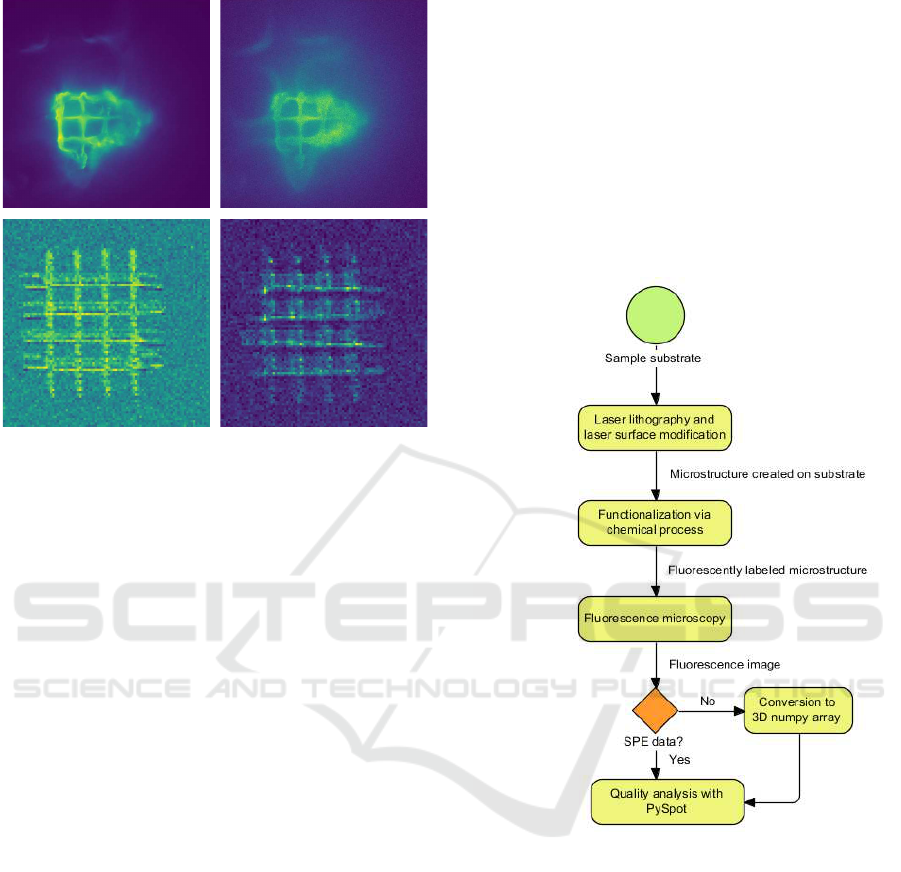
Figure 1: Different images resulting from the workﬂow de-

scribed in the chapter above. (a) and (b) show the result of

2D data, while (c) and (d) show individual layers of a 3D

image.

Figure 1 (a) and (b) show examples of 2D data

received through SPE ﬁles. Those images contain a

grid drawn through the application of laser lithogra-

phy and laser grafting. The images (c) and (d) show

different layers of a 3D microstructure originating

from a 3D Numpy array. (c) shows the third layer

of a structure, and (d) shows the fourth layer. In both

of those images, the intensities are rather low, mak-

ing it difﬁcult to analyze the structure quality without

proper software. Thus, we require an image analy-

sis software to assess the reliability and quality of the

newly created technique. One of the most famous and

widely used image analysis tools is the open-source

processing software ImageJ. Opening and modifying

an image of the SPE format is not possible in the base

version of ImageJ and requires the installation of a

plugin. The 3D Numpy arrays cannot be opened or

modiﬁed with the base version but would require the

implementation of a custom plugin. ImageJ includes

a vast number of functionalities, making it sometimes

too complicated and unsuitable for unfamiliar users.

Another frequently used tool for image analysis is

provided by the computing environment and language

MATLAB and its image processing toolbox. While

MATLAB and its toolbox offer most functionalities

needed for the review, it requires the implementation

of a GUI from scratch and the integration of the spe-

ciﬁc functions. The variety of image formats and the

lack of easy-to-use software for image analysis raised

the need for specialized software. Our software en-

ables loading images in the form of SPE and TIFF

ﬁles, as well as Numpy arrays. Detailed analysis re-

quires image segmentation, edge detection, and the

creation and manipulation of ROIs. To evaluate the

quality of the created image, the information con-

tained inside an ROI’s borders need speciﬁc statisti-

cal evaluation by intensity analysis. PySpot is a user-

friendly graphical interface implemented in Python

for the analysis and evaluation of the 2D and 3D im-

ages. A further advantage is that PySpot is executable

on Windows as well as on Raspbian. PySpots func-

tionality, as well as its methods, are described in detail

in this paper.

Figure 2: Analysis of microstructures using imaging and

image analysis with PySpot.

2 IMPLEMENTATION

PySpot is an image analysis tool implemented in

Python and was created to easily analyze and evaluate

images of 2D and 3D laser-created microstructures,

see Figure 2. PySpot accepts data from SPE ﬁles

created by the Princeton Instruments CCD Cameras,

TIFF ﬁles, as well as in the form of 3D Numpy arrays

for analysis, and all available functionalities work for

all three formats. PySpot provides features for the

creation of regions of interest (ROI) and their analysis

through statistical evaluation. Furthermore, it allows

for the evaluation of the image through thresholding,

BIOIMAGING 2020 - 7th International Conference on Bioimaging

136

edge detection, and surface plots on Windows as well

as on Raspbian.

2.1 Cross-sections

A cross-section is deﬁned as ,,something that has been

cut in half so that you can see the inside or a model

or picture of this.” (Rationality, 2019). In PySpot, a

line represents a cross-section. It provides informa-

tion regarding the intensities of pixels located on the

line representing the cross-section, as well as its coor-

dinates and length. Additionally, a histogram allows

for a simple visualization of the intensity difference

of the respective pixels.

2.2 Region of Interest

A region of interest (ROI) is a subset of an image, that

has been identiﬁed for a particular reason. In connec-

tion with image analysis, an ROI is a speciﬁc section

of an image that marks the region to be analyzed by

the program. In PySpot, an ROI can either be formed

like a rectangle or polygon and give information on

the ROI’s area, dimension, coordinates, and the sta-

tistical evaluation of its containing pixels.

2.3 Automatic ROI Detection

PySpot includes a feature for the automatic detection

of ROIs on the currently displayed image. This fea-

ture uses the principle of thresholding and contour

ﬁnding. Since both algorithms work with grayscale

images, the ﬁrst step consists of converting the dis-

played image from RGBA to grayscale. The resulting

image will be given to a thresholding function to cre-

ate a binary image with the foreground in white and

the background in black, which will then be used to

single out the contours inside the image. The received

contours vary greatly in size and can be as small as

just one pixel. Therefore, each contour below a cer-

tain height and width is singled out. The user chooses

those limits. If a contour meets the requirements, its

points will be saved into an array, added as a new ROI,

and automatically drawn onto the image. In the case

of a 3D image, the ROIs will be searched for in the

currently displayed layer and not for every individual

one. The resulting ROIs created by this step will be

inserted in every layer of the 3D image, resulting in

a way to supervise the change in intensity through-

out the layers.Thresholding is an image segmentation

technique, which isolates certain values on an image

by converting it to a binary image. The image given

to a thresholding function needs to be in a greyscale

format, and its components will then be partitioned

into foreground and background based on their inten-

sity values. Every pixel with a value above a spe-

ciﬁc limit will be assigned a new value. Pixel with a

value equal or below the limit will be assigned a dif-

ferent value (Sahoo P., 1988). A contour is a curved

line, which connects all consecutive points with the

same value along a boundary. In image analysis, con-

tours provide a proper way to get important informa-

tion regarding object representation and image recog-

nition (Satoshi Suzuki, 1985) (Seo J., 2016). Contour

ﬁnding algorithms use binary images with white as

the color for the foreground and black for the back-

ground. Due to this requirement, it is best to convert

the desired image to greyscale and then apply thresh-

olding. Contour ﬁnding algorithms ﬁnd a start point

near a white-black border and from there on track ob-

jects alongside the boundary between the white fore-

ground and black background. The contours coordi-

nates are saved in memory in the respective tracing

order (Satoshi Suzuki, 1985) (Seo J., 2016).

2.4 Deﬁnition of ROI Boundaries

Finding the right borders for ROIs can be quite difﬁ-

cult in certain images. Thus, PySpot includes an edge

detection feature, which will highlight the image’s ob-

ject edges. Edge detection allows for an easy way to

segment an image and visually extract data from it.

This can help in the image analysis and localization

of objects and therefore, the boundaries of potential

ROIs. The edge detection feature uses well-known al-

gorithms like the Gaussian-blur and Canny edge de-

tection. Both of those algorithms require grayscale

images. Hence, the ﬁrst step consists of the image’s

conversion from RGBA to grayscale. Once it has been

converted, it is given to the Canny edge detection al-

gorithm, which uses the discontinuities of brightness

to detect the edges. Due to a great variety in the im-

ages that have to be analyzed, PySpot will automat-

ically display a second edge detection image, which

got smoothed by an additional Gaussian-blur before-

hand. This results in a smoother version of the im-

age and will make small, insigniﬁcant edges and un-

wanted noise disappear from the end-result.

The Gaussian-blur, also called Gaussian-smoothing,

is an image processing technique used to reduce noise

and the amount of detail in an image by smoothing

the intensity differences with the Gaussian function

(Gedraite E., 2011) (Deng G., 1993).

g(x, y) =

2πσ

−

2σ

(1)

PySpot: A Python based Framework for the Assessment of Laser-modiﬁed 3D Microstructures for Windows and Raspbian

137

Due to the property of an image to display a pixel

value as one single value, the equation shown in equa-

tion 1 has to be approximated. The Gaussian-blurs

kernel decides the radius around a pixel in which the

approximation should be realized (Gedraite E., 2011)

(Deng G., 1993). Canny edge detection was devel-

oped by John F. Canny in 1986 and is a widely used

edge detection operation, which works by detecting

an image’s discontinuities in brightness. Edge de-

tection algorithms are used for the segmentation and

data extraction by tracing the boundaries of objects in-

side an image (J., 1986). This algorithm is composed

of ﬁve different steps, which can only be applied to

greyscale images. In the ﬁrst step, the Canny edge

detection algorithm smooths the given image with the

Gaussian-blur function. This results in a smoother

image with less noise, which could be interpreted as

the wrong edges. Afterward, in the second step, four

different ﬁlters are being used to allow the detection

of horizontal, vertical, and diagonal edges. This is

done by applying an edge detection operator on the

image, calculating the ﬁrst derivative in the horizon-

tal or vertical direction. In the next step, the edges of

the image will be thinned out. Therefore, smaller, in-

signiﬁcant edges disappear. This is done by compar-

ing the intensity of each pixel with the next pixel at its

positive and negative gradient direction. If the current

pixels intensity is higher than its neighbor’s, it is be-

ing kept as an edge; otherwise, it will be suppressed.

The edges remaining after this step will be catego-

rized as either ,,strong” or ,,weak” edges based on the

value of their derivatives. To ﬁlter out the remaining

noise and the actual edges, in the last step of the algo-

rithm, pixels marked as weak will be transformed into

strong ones, as long as they are neighbors to at least

one other strong pixel in the image (J., 1986).

2.5 Using Thresholding for Improved

ROI Detection

Even through the use of the automatic ROI detection

feature or the visual boundaries achieved by edge de-

tection, ﬁnding the perfect form and size for an ROI

can be quite difﬁcult. The automatic detection might

not ﬁnd the exact ROIs desired by the user due to a

wrong set of parameters or too much noise in the im-

age. The edge detection functionality cannot always

provide a full outline of the objects, because of in-

tensity ﬂuctuations alongside the border. One way

to improve the detection step and narrow down the

amount of potential ROIs is thresholding. A thresh-

olding functionality sets all pixels of an image to ei-

ther fore- or background based on a limit given by the

user. This creates a sharp edge between the contained

elements and their background, facilitating the pro-

cess of ﬁnding an ROI’s boundary when used as the

base image used for automatic detection.

2.6 Image Rescaling

Images acquired by the workﬂow can vary in size, de-

pending on the use of camera settings and the data to

be analyzed. Thus, using a ﬁxed dimension for the

image displayed by PySpot can be quite tricky, due

to loss in quality. Therefore, images in PySpot are

displayed in their original size. While this works per-

fectly for most images, some images’ original size is

too small to see the elements clearly or to select ROIs

with the utmost precision. Therefore, PySpot includes

a feature to change the size of the images by a speciﬁc

factor between one and ten. A user can freely change

the scaling of the image and zoom in and out as they

wish to. Resizing an image can always be done during

the analysis process. Hence, all elements contained

are adapted to the new size of the image as well.

2.7 Axes Visualization

A 3D image in PySpot is displayed layer by layer,

using a scrollbar to scroll up and down the individ-

ual sections of an image alongside one axis. This al-

lows for an easy way to modify and analyze the cur-

rently displayed axis. As a side-effect, it is not possi-

ble to look at the axes besides the one currently dis-

played, requiring the need for a particular feature to

view all axes simultaneously. The axes visualized are

the XY-axis (which most analysis processes use), the

XZ-axis, and YZ-axis. A new window opens upon

starting the feature to prevent an overﬁlling of the

main window. This requires the implementation of an

entirely new application. This new application con-

tains three individual graphical views for each axis

to be displayed, scrollbars to allow scrolling and a

checkbox to allow switching between a colored and

grayscaled image. Upon opening the application, for

each image alongside an axis, its pixel values are ex-

tracted from the Numpy array. The extracted values

are converted into an image and appended to an ar-

ray of images. This array contains all images of an

axis. This structure allows for an easy way to scroll

through the layers of an axis. Once every image was

converted and saved into its respective array, the ap-

plication opens. Visualizing the axes in a single win-

dow.

BIOIMAGING 2020 - 7th International Conference on Bioimaging

138

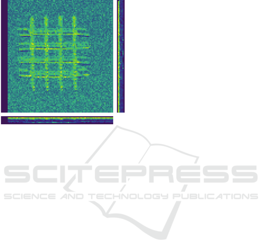
XY YZ

Figure 3: Axes visualization of 3D data. The individual

axes (XY, XZ, YZ) are displayed next to each other, giving

a great overview.

2.8 3D Rendering

Often, it is important to get a 3D understanding of the

construct of a 3D image. This cannot be visualized

simply by looking at the individual layers of the axes.

3D rendering provides an easy way to get a better 3D

understanding of the objects in the image. The 3D

rendering feature in PySpot is based on PyQtGraph,

which relies on PyOpenGL for the 2D and 3D visu-

alization of objects. For this feature, the image ﬁrstly

loaded into PySpot is given to another script as a pa-

rameter. This script creates a new window, which will

contain the 3D render. Information about the image’s

individual pixels is taken and modiﬁed. Through this

modiﬁcation, negative values are removed, and the

overall values smoothed down. This array of mod-

iﬁed pixels is added to a GLViewWidget as an item

and shown as a 3D Render. The initial intensity deter-

mines the representation of the individual pixels. The

user can set a lower and upper limit before creating

the image, which decides the coloration of the pixel

in the 3D rendering. Pixels below the lower limit are

omitted, while green represents those in between the

lower and upper limits. Those above the upper limit

are blue.

2.9 Grayscaling for Improved Intensity

Differentiation

Each color has a different inﬂuence on the way a per-

son perceives an image and its containing objects.

Therefore, PySpot offers functionality to switch be-

tween an image’s colored and grayscaled version.

Colored images provide a better way to visualize the

degree of intensity of the objects of an image, while

grayscaled images offer a better way to analyze and

locate the transition between intensities. To provide

this feature, the loading step of an image creates an ar-

ray for each color scheme. During the next step, each

layer of the loaded image is converted into a colored

RGBA and grayscaled image and saved into the re-

spective array. Through a checkbox in the GUI, a user

can switch between those two color schemes. Allow-

ing the adaptation of the image’s presentation to their

current need.

3 RESULTS

We evaluated the accuracy of the laser manipula-

tion methods used to create 3D microstructures using

PySpot. In the ﬁrst step, an image is loaded into the

program and displayed as an RGBA image. Example

images are shown in Figure 1 (a) and (b) and came

from an SPE ﬁle. Image (a) contains a grid as a car-

rier structure where a small part was modiﬁed using

laser manipulation to add a thin layer that enables the

binding of ﬂuorescence-labeled proteins. Whereas

(b) shows another grid, which has not been modi-

ﬁed. (c) and (d) show the third and fourth layer of

a 3D Numpy array, containing another carrier struc-

ture. The automatic ROI detection feature is used to

mark the important regions for the analysis. It is based

on the principle of thresholding and contour ﬁnding.

Therefore, applying a threshold beforehand provides

an easy way to segment the regions of an image se-

lectively. Also, narrowing down the area signiﬁcant

for ROI detection saves computing time, and unnec-

essary calculations. In Figure 4, a thresholding step

was taken before applying the ROI detection, narrow-

ing down the regions marked. As an alternative to

the thresholding feature, another method used to get a

better understanding of an area’s outline and the bor-

der of potential ROIs is the edge detection feature.

This feature uses a Gaussian-blur and Canny edge de-

tection to ﬁlter out the outlines of an image’s elements

and displays them in two different result windows.

The ﬁrst of those windows contains an edge detection

solely with the Gaussian ﬁlter already implemented

in the Canny algorithm. Therefore, also containing

PySpot: A Python based Framework for the Assessment of Laser-modiﬁed 3D Microstructures for Windows and Raspbian

139

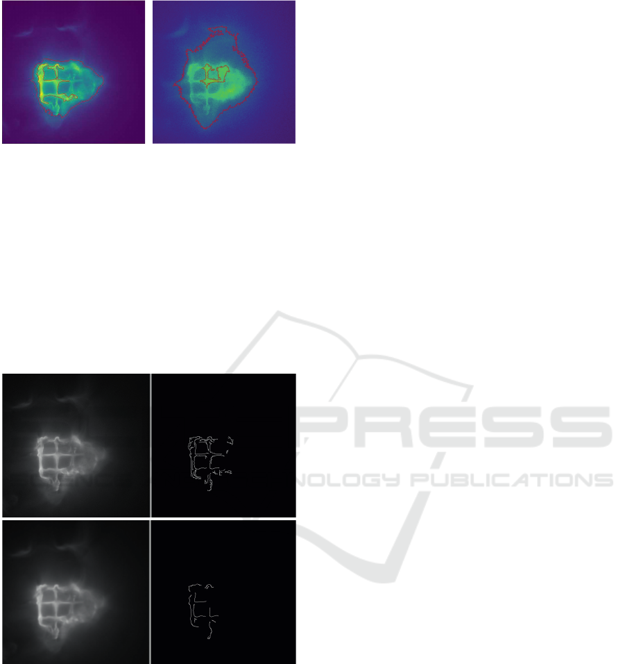
a b

Figure 4: Automatically detected ROIs on the correspond-

ing images from Figure 1. The ROIs in (a) are rather small

and outline the brighter structure almost perfectly. Contrary,

the ROIs in (b) cover a much greater area due to the brighter

background.

the edges of smaller, potentially insigniﬁcant borders.

Thus, the second window displays an image, which

had an additional Gaussian-blur applied to it before

detecting the edges. This results in a smoother in-

put image and fewer detected borders. The user can

determine the parameters used for the Gaussian-blur

and the limits required for the Canny edge detection

algorithm.

Figure 5: Image (a) shows the original image in grayscale

and the result of the Canny edge detection without and extra

blur. In the image (b) a Gaussian-blur was applied before

the edge detection.

As seen in Figure 5, a detection without additional

Gaussian-blur results in more detected edges. Since

most ROIs only need the main outline of an element

and not the small edges in between, this image of-

ten contains too much information. As an alternative,

the image from Figure 5 (b) has had a Gaussian-blur

with a dimension of 5, and a sigma of 3 applied to

it, signiﬁcantly reducing the detected edges. This re-

duces the contained information in the image and will

display an element’s outlines clearer in some cases

than the version with all edges. Since this feature is

solely to get a better understanding of the edges of

the elements, the result is not taken into account dur-

ing an automatic ROI detection. Regardless of the

way, an ROI is drawn, be it automatically or manu-

ally, the evaluation of their pixels is always the same.

First of all, every ROI displays its dimensions and

area, as well as coordinates, in a table as basic in-

formation. Another second table displays informa-

tion about the intensity of all pixels inside an ROI.

This includes the minimum, average, and maximum

intensity of all contained pixels, giving a general view

of the brightness of the marked region. The brighter

an ROI’s intensity, the more particles have accumu-

lated inside its borders. Naturally, the overall inten-

sity of pixels is not enough to evaluate the success

of the cultivation. Therefore, a third table contains

information about each pixel inside of the currently

selected ROI. Each pixels’ intensity is compared to

its background, creating a direct relationship between

its quality and intensity. The ﬁrst comparison made

is on a percentage basis and calculated by dividing

the background’s intensity by the intensity of the par-

ticular pixel, and saved as the contrast of the pixel

to its background. The second comparison is named

Delta and gives the absolute difference between pixel

intensity and background. Histograms visualize the

individual intensities and their frequency in an ROI,

offering a great addition to the statistical evaluation,

due to the qualities connected to the intensities of the

pixels, as seen in Figure 6. The visualization with a

histogram helps in the detection of outliners, which

could have a signiﬁcant inﬂuence on the quality and

evaluation. Through the knowledge of the intensity

distribution, a thresholds limit, and ultimately the out-

lines of an ROI can be set with more precision. As

seen in Figure 6, the results can vary greatly from one

ROI to another. While the ROI in (a) mostly has inten-

sity values around 4.000 counts per pixel, the ROI in

(b) shows much higher overall intensity values, with

the majority ranging between 5.000 and 6.000 counts

per pixel. This shows that segmenting the image with

different thresholds has a great impact on the selected

region’s overall quality. Since the ﬁrst ROI spans

over a greater area than the second one, its intensities

are far more diverse than those concentrated in (b),

taking thinly cultivated regions into account as well.

Through a comparison of (a), (b) with (c), and (d), the

difference between the two analyzed images becomes

prominent. When judging the images with the naked

eye, the difference between the images does not seem

too severe. Through comparison of the images with

BIOIMAGING 2020 - 7th International Conference on Bioimaging

140

a b

c d

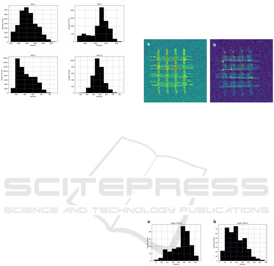
Figure 6: Histograms of the biggest ROIs in Figure 4, y-axis

displays the number of pixels and the x-axis the different

intensities. (a) and (b) show the histograms for the ROIs

outlined in Figure 4 (a). (c) and (b) those outlined in Figure

4 (b). (a) and (c) contain the intensities of the big ROIs

created with a threshold of 100, and (b) and (d) those of the

smaller ROIs.

the program, the major difference becomes clear. The

ROI on Figure 4 (a) is around ten times higher than

those in (b).

All those steps can be taken with 3D images, as

well. Visualizing the difference between the individ-

ual layers of a 3D area created through later modi-

ﬁcation. The ﬁrst step consisted of a grayscale con-

version to get a better understanding of the individual

transitions between fore- and background. Afterward,

thresholding is applied to the image to segment the

previously found structures. The result of this step

can vary greatly among layers. This variation can be

due to the quality of the modiﬁcation on the different

layers, causing particles to more prominently accu-

mulate on one layer than another. While this might

be the case for several layers in some images, oth-

ers only contain one layer with such a great differ-

ence and show certain outliners. This makes the se-

lection of a matching ROI quite difﬁcult since there

is no complete consistency in the present data. Due

to this inconsistency among some layers, the layer

chosen for an automatic ROI detection has a great in-

ﬂuence on the resulting quality evaluation of the im-

age. Figure 7 shows the biggest ROI resulting from

an automatic detection on layer three with a threshold

limit of 150. As seen in the ﬁgure, the shown ROI

includes many pixels with an intensity above 150 on

layer three, while it contains almost no pixels above

this value on layer four. Visualizing the great differ-

ence in intensity and density of ﬂuorescent particles

on those two layers. Choosing another layer as the

base for the detection, the resulting ROI would have

marked a different area. Therefore, the layer chosen

for the detection determines the main feature of the

quality evaluation of the whole 3D image. The great

difference is even more evident in the statistical eval-

uation of the ROI’s pixel values, as seen in the his-

tograms of Figure 8.

Figure 7: Automatically detected ROIs with threshold limit

150 on layer 3 in (a) and layer 4 in (b).

The intensity of the contained pixels varies greatly

between the layers. On layer three, most of the con-

tained pixels show an intensity value of 180 counts

per pixel, with the majority collecting around 200

and the highest going up to just above 250 counts

per pixel. Contrary to this, the pixels on layer four

show a way lower intensity, with values ranging be-

tween 5 and 160. The largest share shows an intensity

of around 40 counts per pixel, with an average of 58

counts per pixel. While the histograms show the dis-

tribution of counts per pixel, the statistical evaluation

is provided by different tables in the same way as for

the 2D data.

Figure 8: Histograms of the ROI shown in Figure 7. The

y-axis displays pixel quantitiy and the x-axis intensities. (a)

displays the values of layer three, while layer four is repre-

sented in (b).

Retrieving all necessary information out of a 2D rep-

resentation is often difﬁcult and also does not provide

the visualization needed to get a proper understanding

of the current 3D structure. Therefore, the 3D render-

ing can be used to get a more natural visualization of

the data, as seen in Figure 9. The visualized data is

placed on top of a grid, which functions as a base and

helps in judging the datas dimension.

PySpot: A Python based Framework for the Assessment of Laser-modiﬁed 3D Microstructures for Windows and Raspbian

141

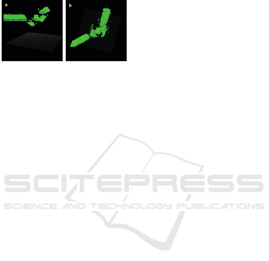
Figure 9: 3D rendering of a hair knot with a lower limit of

65 and an upper limit of 80. (a) shows the rendered image

from the side, while (b) shows the top view.

4 CONCLUSION

In this paper, we show an easy-to-use software for

analyzing and evaluating SPE, TIFF, and Numpy ar-

ray data. The features of the software were illustrated

using 2D and 3D imaged microstructures. PySpot

provides standard functionalities, e.g., histograms and

thresholding and even more specialized features like

automated detection of ROIs and visualization of

three orthogonal layers (XY, XZ, and YZ) in one ﬁg-

ure. For improved analysis of 3D data, functionalities

for the tracking of individual pixels’ intensities or an

improved 3D rendering with the option of data ex-

traction can be implemented in the program. Since

Python is an interpreter language, PySpot is not as

fast during calculations and operations as other image

analysis software packages. Instead, its beneﬁts lie in

its simplicity, compatibility with different operating

systems, and easy adaptability. There is the possi-

bility to use it on Windows as well as on Raspbian.

Therefore, it can be used on a Raspberry Pi, which

are cheap, single-board computers. Additionally, this

basis allows for an easy way to add self-implemented

features into the program, adapting it to individual re-

quirements and different types of data. PySpot can

be downloaded free of charge at the homepage of the

Bioinformatics Research Group Hagenberg (http:

//bioinformatics.fh-hagenberg.at). Due to its

simplicity, yet vast array of functionalities, PySpot is

suited for inexperienced as well as experienced users.

ACKNOWLEDGEMENTS

This work was funded within the TIMED Center

for Technical Innovations in Medicine of the Univer-

sity of Applied Sciences Upper Austria (TC-LOEM)

and by the Basic Research Funding Program of the

University of Applied Sciences Upper Austria (AB-

SAOS).

REFERENCES

Buchegger B., Vidal C., N. J. B. B. K. A. H. A. K. T. A.

J. J. (2019). Gold nanoislands grown on multiphoton

polymerized structures as substrate for enzymatic re-

actions. ACS Materials Letters, pages 399–403.

Deng G., C. L. (1993). An adaptive gaussian ﬁlter for noise

reduction and edge detection. volume 3, pages 1615 –

1619.

Gedraite E., H. M. (2011). Investigation on the effect of

a gaussian blur in image ﬁltering and segmentation.

pages 393–396.

J., C. F. (1986). A computational approach to edge detec-

tion. IEEE Transactions on Pattern Analysis and Ma-

chine Intelligence, PAMI-8:679–698.

Kawata S., Sun H.-B., T. T. T. K. (2001). Finer features for

functional microdevices. Nature, 412(6848):697–698.

Maruo S., Nakamura O., K. S. (1997). Three-dimensional

microfabrication with two-photon-absorbed pho-

topolymerization. Opt. Lett., 22(2):132–134.

Ovsianikov A., Li Z., T. J. S. J. L. R. (2012). Selective func-

tionalization of 3d matrices via multiphoton grafting

and subsequent click chemistry. Advanced Functional

Materials, 22(16):3429–3433.

Rationality (2019). The Cambridge Dictionary.

Sahoo P., Soltani S. and, W. A. (1988). A survey of thresh-

olding techniques. Computer Vision, Graphics, and

Image Processing, 41:233–260.

Satoshi Suzuki, K. A. (1985). Topological structural anal-

ysis of digitized binary images by border following.

Computer Vision, Graphics, and Image Processing,

30(1):32 – 46.

Seo J., Chae S., S. J. K. D. C. C. H. T. (2016).

Fast Contour-Tracing Algorithm Based on a Pixel-

Following Method for Image Sensors.

Wollhofen R., Buchegger B., E. C. J. J. K. J. K. T. A. (2017).

Functional photoresists for sub-diffraction stimulated

emission depletion lithography. Opt. Mater. Express,

7(7):2538–2559.

BIOIMAGING 2020 - 7th International Conference on Bioimaging

142