Combining Image and Caption Analysis for Classifying Charts in

Biodiversity Texts

Pawandeep Kaur

1 a

and Dora Kiesel

2 b

Heinz-Nixdorf Chair for Distributed Information Systems, Friedrich Schiller University, Jena, Germany

Bauhaus University, Faculty of Media, VR Group, Weimar, Germany

Keywords:

Caption Analysis, Chart Classiﬁcation, Natural Language Processing, NLP, Caption Classiﬁcation, Visualiza-

tion Recommendation, Chart Recognition

Abstract:

Chart type classiﬁcation through caption analysis is a new area of study. Distinct keywords in the captions

that relate to the visualization vocabulary (e.g., for scatterplot: dot, y-axis, x-axis, bubble) and keywords from

the speciﬁc domain (e.g., species richness, species abundance, phylogenetic associations in the case of biodi-

versity research), serve as parameters to train a text classiﬁer. For better chart comprehensibility, along with

the visual characteristics of the chart, a classiﬁer should also understand these parameters well. Such concep-

tual/semantic chart classiﬁers then will not only be useful for chart classiﬁcation purposes but also for other

visualization studies. One of the applications of such a classiﬁer is in the creation of the domain knowledge-

assisted visualization recommendation system, where these text classiﬁers can provide the recommendation

of visualization types based on the classiﬁcation of the text provided along with the dataset. Motivated by this

use case, in this paper, we have explored our idea of semantic chart classiﬁers. We have taken the assistance

of state-of-the-art natural language processing (NLP) and computer vision algorithms to create a biodiversity

domain-based visualization classiﬁer. With an average test accuracy (F1-score) of 92.2% over all 15 classes,

we can prove that our classiﬁers can differentiate between different chart types conceptually and visually.

1 INTRODUCTION

Automatic chart type classiﬁcation is an increasingly

common pursuit in visualization. In the majority of

cases, the overall goal of the chart classiﬁcation is au-

tomatic chart comprehension. Nonetheless, previous

studies (Liu et al., 2013),(Abhijit Balaji, 2018),(Savva

et al., 2011),(Jobin et al., 2019) have paid little at-

tention to the role of the free text information pro-

vided along with the charts in the form of captions.

Processing only the visual chart elements in the im-

age can recognize the type of chart well, however,

this recognition alone is not enough to understand

the chart semantics. Captions on the other hand pro-

vide clear goals of the represented charts and resolve

the ambiguity that arises due to visually similar chart

types. For example, column charts look similar to

histograms but their representative goals are differ-

ent. Column charts are used to represent the com-

parison among various sizes of the data series while

histograms show the frequency with which speciﬁc

https://orcid.org/0000-0002-3073-326X

https://orcid.org/0000-0002-6283-2633

values occur in the dataset (Harris, 2000). Due to the

different chart semantics, an image classiﬁer alone,

which might decode a histogram as a column chart

would not be able to provide an accurate and efﬁcient

automatic interpretation.

After manually surveying a vast number of cap-

tion samples during the corpus creation process, we

know that chart captions provide information about

a) representative goals of the author which are not

directly visible from the image itself, b) domain-

speciﬁc tasks, depicted through the chart and c) chart

layout and pictorial elements (e.g. text, colors, lines,

shapes). Consider, for instance, Figure 1 and the orig-

inal caption to the visualization depicted in Figure 1

(Moody and Jones, 2000).

”Fig. 5. Boxplots comparing the distribution of

the measured soil variables at the different canopy

positions at trunk, midcanopy, the canopy edge, and

outside the canopy, respectively. The upper and lower

boundaries of each box represent the interquartile

distance (IQD). The horizontal midline is the median

value. The whiskers extend to 1.5x IQD. Outliers are

displayed as horizontal lines beyond the range of the

Kaur, P. and Kiesel, D.

Combining Image and Caption Analysis for Classifying Charts in Biodiversity Texts.

DOI: 10.5220/0008946701570168

In Proceedings of the 15th International Joint Conference on Computer Vision, Imaging and Computer Graphics Theory and Applications (VISIGRAPP 2020) - Volume 3: IVAPP, pages

157-168

ISBN: 978-989-758-402-2; ISSN: 2184-4321

157

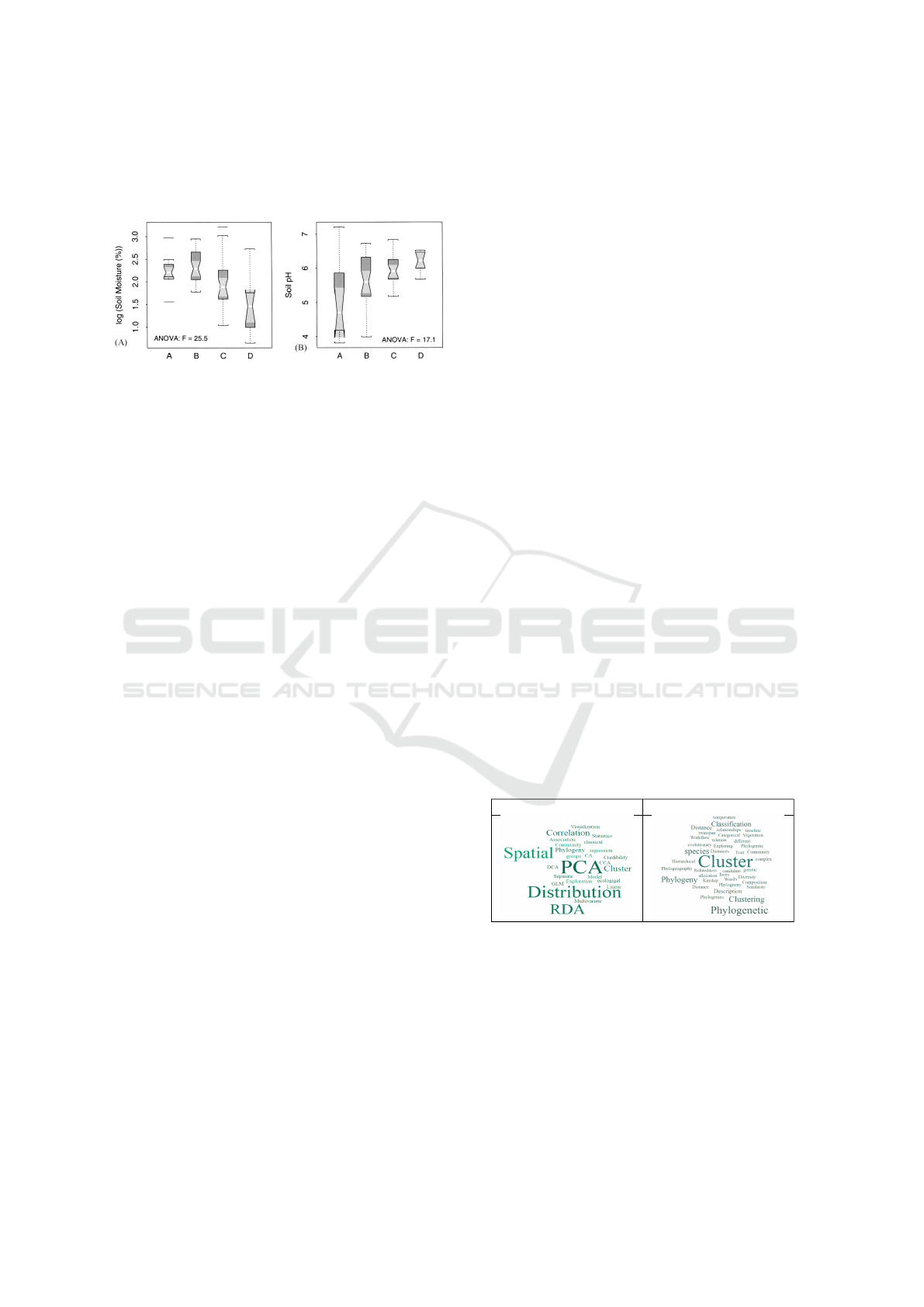
whiskers. If the notches of any two boxes do not over-

lap vertically, this suggests a signiﬁcant difference at

a rough 5% conﬁdence interval.”

Figure 1: Example image adapted from a biodiversity pub-

lication (Moody and Jones, 2000).

The caption of this ﬁgure provides clues about the

following information:

Chart Type: Boxplots, box, horizontal midline,

whiskers, horizontal lines, notches.

Representative Goals: comparing, distribution.

Domain Speciﬁc Variables: soil variables, canopy

positions, trunk, midcanopy, canopy edge.

Statistical or Analytic Information: interquartile

distance (IQD), median value, conﬁdence

interval.

These identiﬁers can serve as important features

for a text classiﬁer.

In this work, we have taken the assistance of both

computer vision and NLP technology in the produc-

tion of a very ﬁrst text classiﬁer that identiﬁes the best

ﬁtting chart from a set of ﬁfteen different chart types

given a biodiversity caption or data description. The

classiﬁer was incrementally trained, starting with a

dataset of 4073 manually annotated biodiversity vi-

sualization captions and achieves an average test ac-

curacy (F1-score) of 92.2% over all 15 classes. The

classiﬁer understands a speciﬁc chart vocabulary and

related biodiversity vocabulary used for each partic-

ular chart type and will, therefore, only work on the

biodiversity text. However, the described workﬂow

can be used to train classiﬁers for other different do-

mains as well.

Our primary contribution is the chart classiﬁcation

workﬂow that classiﬁes a chart not only on the basis

of chart elements in the image but also on the basis of

captions. Following this workﬂow creates a semantic

chart classiﬁer that understands the visualization type

along with the high level visualization goals. We also

contribute by providing a novice approach in the ﬁeld

of data visualization recommendation system, to rec-

ommend visualization schema via visualization clas-

siﬁer based on the knowledge gathered at the train-

ing process. In our knowledge, we are the ﬁrst who

conceptualize and implement a visualization classiﬁer

that understands the semantics of the chart and can

infer representative goals from the biodiversity text

based on the different chart types.

In Section 2 we present the motivation for this

work, state-of-the-art in Section 3, classiﬁcation pro-

cess is presented in Section 4, result and discussion in

Section 5, challenges and research directions in Sec-

tion 6 and conclusion in Section 7.

2 MOTIVATION

The chart type classiﬁcation we present in this pa-

per will constitute one important step in a biodiver-

sity knowledge-assisted visualization recommenda-

tion system that will suggest suitable visualization

types based on biodiversity research data and goals.

To build such a system, a visualization designer

needs to know the domain-based and the visual goals

of the user (Munzer, 2009). In the earlier stages of our

study, we tried to gather this information via a survey.

Due to the limited responses, we could not get good

representatives of the dataset. An excerpt of the re-

sult is shown in Table 1. It shows that scientists use

scatterplot prominently to convey the result of differ-

ent ordination analysis techniques (PCA, RDA, DA)

and Dendrogram is more prominently used to rep-

resent Phylogeny, Classiﬁcation and Clustering. To

gather this knowledge in bulk and to use this knowl-

edge to classify future biodiversity texts serve as the

main motivation in the creation of biodiversity visual-

ization classiﬁer.

Table 1: Visualization types and the purposes they are used

for in biodiversity domain (Kaur et al., 2018).

Scatterplot Dendrogram

The proposed system, depicted in Figure 2, will

work as follows: After the user provides a data table

and a description of its contents, along with how it

was created, its intended research goals, and so forth,

a biodiversity visualization text classiﬁer is applied to

suggest the most suitable visualization types to rep-

resent the data based on its vast knowledge of similar

data and research goals. In a second step, based on the

visualization type, our context-aware algorithm will

select the suitable data variables that can be mapped

IVAPP 2020 - 11th International Conference on Information Visualization Theory and Applications

158

to the visualization.

The goal of the chart type classiﬁcation task de-

scribed in this paper is the creation of a knowledge

base for and the training of the biodiversity text clas-

siﬁer that will be responsible for inferring the best

suited chart types from given metadata text which

provides information about the what and why of the

dataset. The biodiversity text classiﬁer will output a

’predicted visualization list’, which is a ranked list of

suitable chart types for this dataset and related vocab-

ulary. This information can then be used by scientists

to create suitable visualizations and gain new insights

into the selected dataset.

In this paper, we will focus on the creation of the

biodiversity visualization text classiﬁer.

3 STATE OF THE ART

In this section, we present the state of the art of chart

image classiﬁcation and image caption analysis.

3.1 Chart Image Classiﬁcation

Many studies have used different computer vision al-

gorithms for the classiﬁcation of chart types from dig-

ital images. Typical representative of them are Ta-

ble 2. We have found our study different from them

in the following aspects:

• Data Source: We have found that some studies

have used automatically generated synthetic data

(Abhijit Balaji, 2018) and others have used well

curated data from previous studies (Jung et al.,

2017). In their work, (Savva et al., 2011) have

carefully downloaded their dataset from online

search. The resulting dataset does not really re-

ﬂect reality, where intra-class variation is a lot

higher. In our work, we tried to reﬂect this by

creating our corpus from scientiﬁc publications

which have huge intra-class variations (see Ta-

ble 3). Moreover, we have considered various

forms of different charts by grouping them not

only based on their visual similarities but also on

their chart semantics.

• Visualization Classes: The range of the classes

that we have considered (15) is much larger than

most of the previous studies, except (Jobin et al.,

2019), who have also considered other document

ﬁgure types as their classes. Moreover, their train-

ing dataset was far more balanced than what we

had. In our case, we were not aware of the types

of visualizations available in the downloaded cor-

pus in advance. Therefore, it was important for

us to include as many different visualization types

as possible in our training set. This leads to the

assignment of unequal proportion of examples for

many classes.

Table 2: A summary of different chart image classiﬁcation

studies.

Name Year Data source Classes Accuracy

(Savva et al., 2011) 2011 Online 10 96%

(Jung et al., 2017) 2017 Online 10 76,7%

(Abhijit Balaji, 2018) 2018 Synthetic 5 99,72%

(Jobin et al., 2019) 2019 Conferences 28 92,86%

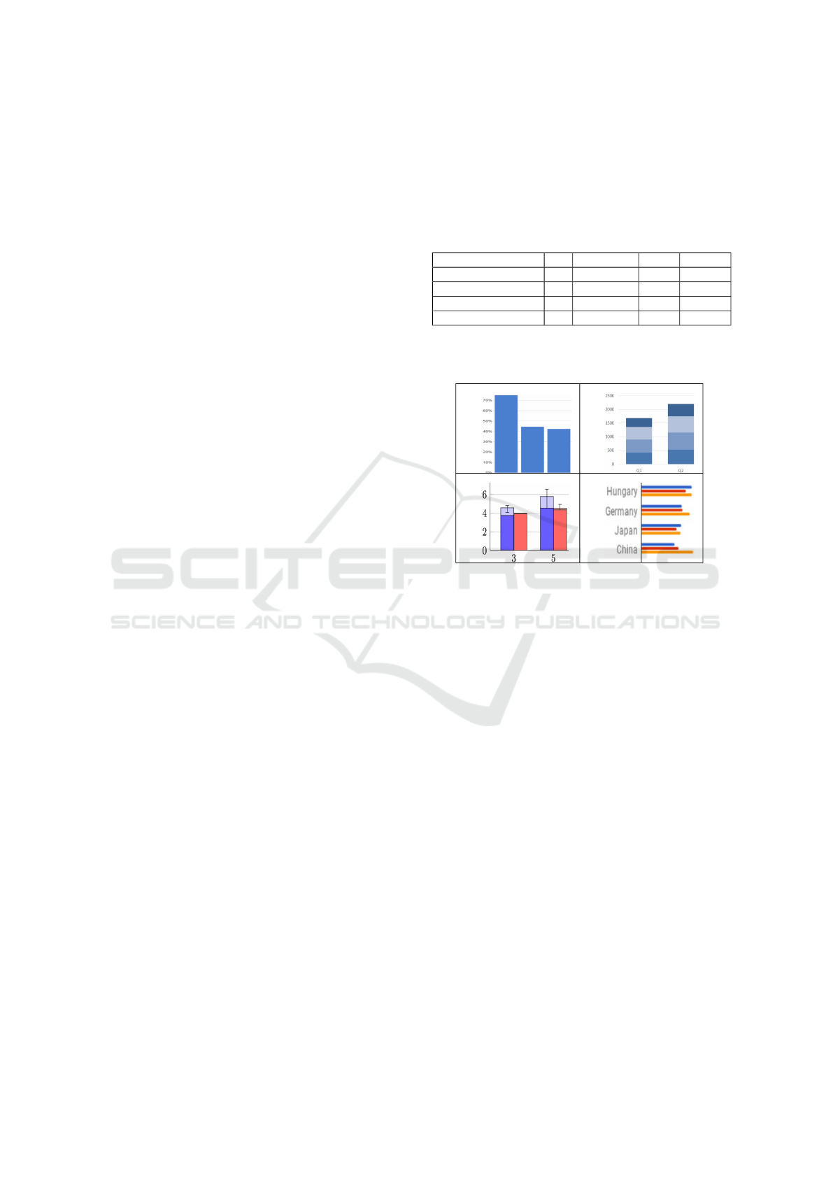
Table 3: Intra-class visual similarity for different variation

of Column or Bar Chart.

(A) (B)

We consider our work to be closed to (Jobin et al.,

2019), who has also done scientiﬁc document ﬁgure

classiﬁcation on publications from different confer-

ences. They had also created their categories based

on what was available to them in their downloaded

corpus. Like us, they pre-selected the categories,

grouped them into super classes and then had used it-

erative learning to gather more trained data. However,

for their classiﬁcation process, they had considered all

different types of ﬁgures available in scientiﬁc docu-

ments, whereas our work is limited to visualization

images only. They have only considered image clas-

siﬁcation, whereas we have taken the beneﬁts of both

text and image classiﬁers for semantically classifying

the visualization types.

3.2 Use of Captions for Classiﬁcation

Purposes

Image captions are an important source of informa-

tion and have been a long-studied subject in differ-

ent domains. Earlier studies have used captions with

computer vision algorithms to identify human faces

in the newspapers (Srihari, 1991). Caption analysis

has been predominantly used in biomedical domain

for its various research goals. In their study, (Murphy

Combining Image and Caption Analysis for Classifying Charts in Biodiversity Texts

159

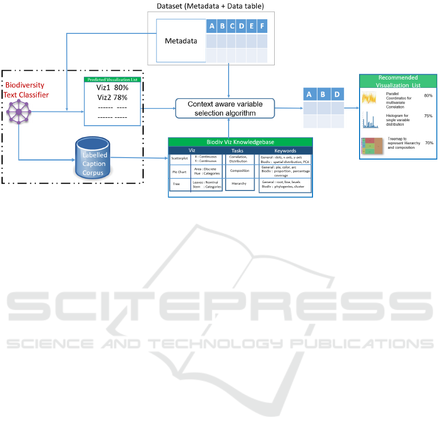
Figure 2: A conceptual diagram of biodiversity knowledge-assisted visualization recommendation system.

et al., 2004) used joint caption image features in clas-

sifying protein sub-cellular location in images. The

study by (Rafkind et al., 2006) was the ﬁrst to use

text identiﬁers from biomedical image captions (”di-

ameter”, ”gene-expression”, ”histogram” etc) to iden-

tify graph chart images as a separate category from

other biomedical image categories. More recent stud-

ies have utilized the information from the captions in

biological documents for the purpose of image index-

ing and search (Charbonnier et al., 2018; Xu et al.,

2008; Lee et al., 2017). So far, caption data has been

used along with the computer vision algorithms to

distinguish graph images from others, however, we

could not ﬁnd any study that has used caption data

alone or caption data in conjunction with other me-

dia, to classify different chart types. Classifying chart

types from caption data is still in a novice state. We

have observed different use cases in which research in

caption analysis could be beneﬁcial for visualization

as well as for linguistics research:

• Visualization Research: The foremost is in the

creation of domain speciﬁc visualization knowl-

edgebases or corpus, 2) a machine learning

model trained on the visualization captions can be

evolved and reused by other users for different do-

main knowledge-assisted visualization products,

3) a text classiﬁer trained on different chart types

can be used for tagging, indexing and searching

visualization documents, 4) it could be a valuable

source for future theoretical visualization research

problems (Chen et al., 2017) like the creation of

visualization ontologies on the basis of classiﬁed

visualization concepts.

• Computer Linguistics Research: Research on

caption classiﬁcation will help 1) to better under-

stand the requirements of classiﬁcations on very

short and convoluted texts, 2) to study the inﬂu-

ence of domain speciﬁc language on classiﬁca-

tion and possibly exploit domain speciﬁc regulari-

ties to improve classiﬁcation results and 3) to ﬁnd

effective ways to integrate domain expert knowl-

edge into the classiﬁcation process.

4 CLASSIFICATION PROCESS

The process of creating the biodiversity text classiﬁer

consists of a sequence of complex steps, visualized

in Figure 3. In order to reach the highest possible

quality in recognizing the best suited chart types from

biodiversity text – e.g. biodiversity image captions

– the underlying training corpus needs to have a suf-

ﬁcient size (we estimated at least 15 000 samples to

be enough, ideally 1 000 for each of the 15 classes)

and quality. So, the ﬁrst step was to manually create

a starting dataset, that associates caption texts with

their respective chart types. This set is then incremen-

tally extended using a combination of image and cap-

tion classiﬁcation in order to gain the highest possible

quality on the automatic labeling of unlabeled data.

The resulting dataset is then used as training set for

the biodiversity text classiﬁer, that can be integrated

into the biodiversity knowledge assisted visualization

recommendation system described in Section 2.

IVAPP 2020 - 11th International Conference on Information Visualization Theory and Applications

160

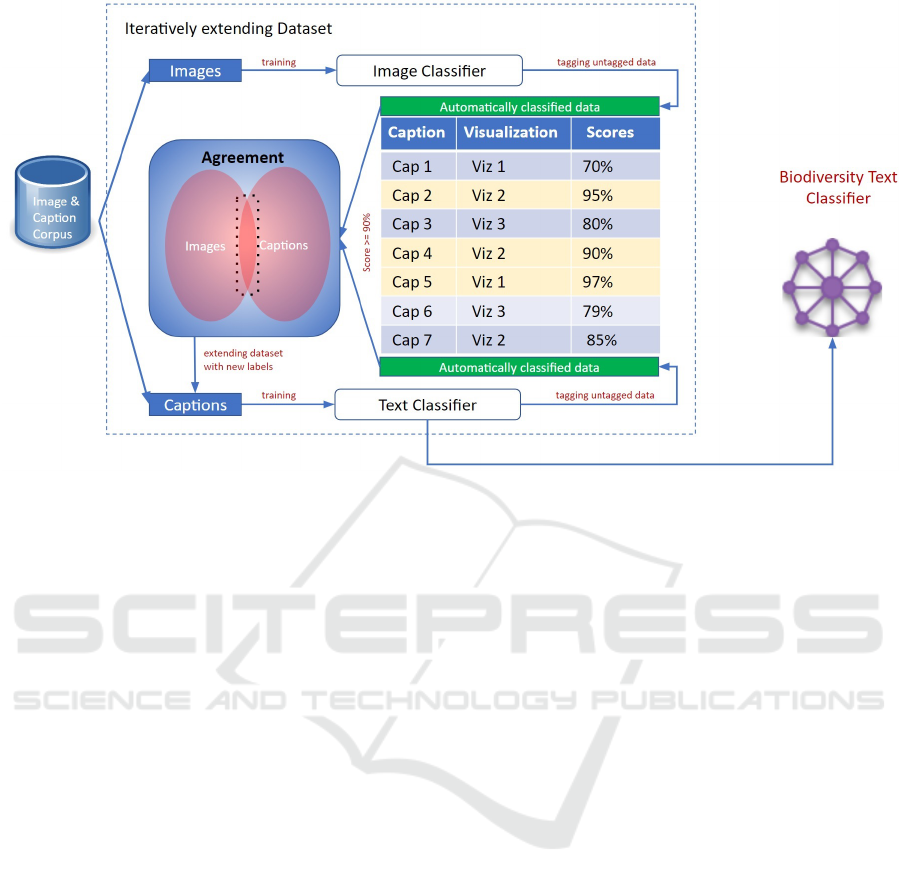
Figure 3: Workﬂow for the creation of the biodiversity visualization text classiﬁer.

4.1 Data Preparation

In our data collection process, ﬁrst we selected the

reputed biodiversity journals which represents differ-

ent biodiversity sub-domains. For details please re-

fer to Section 2 of appendix. We had downloaded

all available volumes and issues of these journals till

2016 which is the year when this download was done.

For creating the initial dataset, we downloaded 26 588

biodiversity publications through Elsevier ScienceDi-

rect article retrieval API (api, 2018), which allows

the download of a complete publication in an XML

format. From these 26 588 downloaded publications,

96 837 images and their captions were extracted using

a python script.

4.1.1 Class Formation and Annotation Process

Out of 96 837 image and caption samples, we cre-

ated our training data by randomly selecting a sub-

set of 4 073 visualization image captions and labeling

them with their respective visualization types manu-

ally. The labelling task was done by one of the author

of this paper who is a Ph.D. student in data visual-

ization with four years of experience in this domain.

In case of disambiguation regarding the selection of

the visualization label for a particular caption, ade-

quate guidance from visualization publications and

reference books (Harris, 2000) was taken. Due to

the sheer richness of different visualization types –

a closer study revealed the sample to contain 59 dif-

ferent visualizations (see Section 1 of appendix) –

we continued our annotation process in the following

stages:

Class Grouping: In order to gain adequate sample

sizes for each of the visualization types or classes, we

split / merged the original 59 classes into super / sub

classes:

> 50 Samples in Class: Since we considered 50 ex-

amples to be sufﬁcient for classiﬁcation, all

classes with same or more examples were kept as

a super classes.

< 10 Samples in Class: These classes had very

small set of examples and were not suitable

match for our super classes. Therefore, they were

rejected from the further annotation process.

All Other Classes: All classes, that do not ﬁgure fre-

quently enough to sufﬁce for the classiﬁcation

task have been merged into super classes either

based on their visual similarity or their represen-

tational goals. For example, chart types that use

the same coordinate space (e.g. xy plot) and same

visual marks (e.g. bars) were considered visually

similar and then were merged. This way, all the

chart types which are visually similar to Column

Chart e.g. Bar Chart, Stacked Bar Chart, Multiset

Bar Chart etc. were all merged into the super class

Column Chart.

On the other hand, Chord Diagrams, Alluvial Dia-

grams and Network diagrams are visually dissim-

ilar but have the common representational goal of

connecting entities. Same with the Pie Chart and

Stacked Area Chart which are visually dissimilar

Combining Image and Caption Analysis for Classifying Charts in Biodiversity Texts

161

but represent a common visual goal of represent-

ing proportion or composition among data enti-

ties.

Thus, they all were grouped in the class ’Net-

work’. All non-visualization images (e.g.,

camera-clicked pictures, conceptual diagrams

etc.) were grouped into the ’NoViz’ class. Due to

the variant structure of non-visualization images,

NoViz class was also excluded from the image

classiﬁcation process. An overview of retained

classes are provided in Section 3 of appendix.

Doing so, we ended up with 15 different super

classes.

Assignment of Classes for Caption Classiﬁcation:

Once, we had formed the classes, we did another

round of annotation. We have now labelled our se-

lected corpus of 4 073 captions with these 15 classes.

For detailed information about these classes, refer to

Section 4 of appendix.

Assignment of Classes for Image Classiﬁcation:

All classes were considered for image classiﬁcation

except for those which are visually similar to other

classes. Histogram is visually similar to the column

chart and timeseries is visually similar to the line

chart (see appendix 3). Thus, histogram and time-

series were ignored from the image classiﬁcation pro-

cess. Alongside, due to the variant structure of non-

visualization images, ’NoViz’ class was also excluded

from the image classiﬁcation process.

We have provided the frequency distribution of

classes for image and caption classiﬁcation in Table 4.

In appendix Section 4, we provide examples for each

class, that consist of the replicated original image and

caption from open-access publications. Due to the

amples from our dataset.

4.2 Image Classiﬁcation

4.2.1 Image Classiﬁcation Model

For image classiﬁcation, we have used Convolutional

Neural Networks (CNNs). CNNs are a specialized

kind of neural networks for processing data that has a

known grid-like topology. Since images can also be

thought as 2D-grid of pictures, thus CNNs have been

tremendously successful in application to image data

(Goodfellow et al., 2016).

For training, we have used reusable pre-trained

neural network modules provided by Tensorﬂow Hub

(TFH, 2019). TensorFlow Hub is a library for the pub-

lication, discovery, and consumption of reusable parts

of machine learning models.

Table 4: Frequency distribution of our manually annotated

training dataset for Caption and Image classiﬁcation.

Classes Caption Classes Image Classes

Ordination Plot 503 278

Map 529 277

Scatterplot 399 272

Line Chart 320 283

Dendrogram 282 243

Column Chart 427 302

Heatmap 147 124

Boxplot 210 104

Area Chart 159 95

Network 58 32

Histogram 57 -

Timeseries 319 -

Noviz 511 -

Pie Chart - 134

Proportion 157 -

Total 4073 2144

Out of the available CNN modules in TFHub, we

chose MobileNet V2 (Sandler et al., 2018) as our

CNN architecture. MobileNet V2 is a family of neu-

ral network architectures for efﬁcient on-device im-

age classiﬁcation and related tasks.

Mobilenet

v2 module of Tensorﬂow Hub contains

a trained instance of the network, packaged to do

the image classiﬁcation. This Tensorﬂow Hub mod-

ule uses the Tendorﬂow Slim implementation of ’Mo-

bilenet v2’ with a depth multiplier of 1.0 and an in-

put size of 224x224 pixels. For training the classiﬁer

we used Keras (Chollet et al., 2015) with Tensorﬂow

(Abadi et al., 2016) backend. To train the classiﬁca-

tion network on our data, we resized the images to

a ﬁxed size of 224 x 224 x 3 and normalized them

before feeding into the network. We used Adam op-

timizing function (Kingma and Ba, 2014) with the

learning rate of 0.001.

4.2.2 Results from Image Classiﬁcation

For evaluation, we have used Keras’ in-build evalu-

ation function. When provided with the suitable pa-

rameters, Keras seperates and retains a portion from

the training data and then uses that unseen retained

data for evaluating the model. For evaluating our

image model, 20% of the examples from the image

dataset were retained from training. Our model has

achieved a classiﬁcation accuracy of 75% on automat-

ically selected batch of 100 images. Then this classi-

ﬁer was used to classify the original corpus of 96837

IDs. Our image classiﬁer was able to annotate 54%,

i.e., 52921 IDs out of 96837 IDs, with the conﬁdence

interval of 95% and more.

IVAPP 2020 - 11th International Conference on Information Visualization Theory and Applications

162

4.3 Caption Classiﬁcation

The 4 073 manually labeled image captions served as

training set for the initial supervised classiﬁer. In or-

der to be able to optimize the classiﬁer for each of the

identiﬁed classes separately, we decided to build bi-

nary classiﬁers, that can distinguish one speciﬁc class

from all others. From these specialized binary clas-

siﬁers an assembly classiﬁer is constructed (see Fig-

ure 4, Training Step). Given an input, the assembly

asks each classiﬁer to process the input separately (as

detailed in Figure 4, Classiﬁcation Step), and receives

a probability score that states how likely it is, that the

given sample is of the respective class. The classes of

all classiﬁers, that give a positive response with a cer-

tain preset conﬁdence (in our case usually 90%), will

then be returned as result vector.

Figure 4: Workﬂow for the creation of the biodiversity vi-

sualization text classiﬁer.

To ﬁnd out which binary classiﬁers to incorpo-

rate into the assembly, we implemented and opti-

mized three standard classiﬁers in text classiﬁcation

(Joachims, 1998; Sebastiani, 2002): Support Vector

Machines (SVM), CNN and Random Forests. SVMs

(Cortes and Vapnik, 1995) are inherently binary su-

pervised learners. In their linear form, they ﬁnd the

maximum-margin hyperplane in data space that best

separates the data points of one class from the data

points of the other class. Kernels (Boser et al., 1992)

have been introduced to generalize the principle to

polynomial, radial or sigmoid functions. Random

Forests (Ho, 1995) are a assemblies of a – usually

rather large – number of Decision Trees that con-

tribute to the main decision in form of a majority

vote. Additionally, in resemblance to the image clas-

siﬁer, a neural network solution – speciﬁcally a mul-

tilayer perceptron classiﬁer with the same stochastic

gradient-based optimizer as the image classiﬁer and

the same constant learning rate of 0.001 – was used.

4.3.1 Preprocessing

As is standard in natural language processing (Aggar-

wal and Zhai, 2012), the labels have been broken into

tokens, stemmed and stop words have been removed

before processing them. Additionally, some standard

phrases that have been identiﬁed during manual n-

gram evaluation of the data and are unrelated to the

contents of the image, like phrases to make people

aware of the modalities of the online version of the

paper – e. g. ”For interpretation of the references

to color in this ﬁgure legend, the reader is referred to

the web version of this article”)– , have been automat-

ically removed. In order to keep the training data as

pure as possible, captions referring to multiple visual-

izations were ﬁltered out, leaving a dataset of 4 066.

The resulting word vectors contain the term fre-

quency - inverse document frequency (tf-idf) scores

(Ramos et al., 2003) per word.

4.3.2 Model Optimization or Parameterization

Each binary classiﬁer has been trained separately on

a data set consisting of all samples of the target class

and an equal number of samples uniformly distributed

over all other classes. Classiﬁers have been evaluated

using a 5-fold-cross-validation, that splits the data set

into 5 equal parts training on 4 parts and testing on

the last. The ﬁnal evaluation result constitutes as the

average of all ﬁve runs.

In order to reach the best results, we optimized

both the pre-processing of the data as well as the pa-

rameters of the classiﬁer itself. On data level, we op-

timized the maximum size of the vocabulary, the min-

imum number of documents each word ﬁgures in and

which n-grams should be included into the analysis.

Applying an exhaustive grid search over the range of

sensible parameters for each feature (vocabulary size:

[250 to 1250 (steps of 250)], minimum document fre-

quency: [0 to 4], n-grams: [1 to 6]), we achieved the

best results using a base vocabulary that consists of

the 750 most important words and 2-grams, that oc-

cur in at least 3 documents in the whole corpus.

We also optimized SVM for its kernel function

(linear, polygonal, sigmoid, and radial basis func-

tion), ﬁnding a linear kernel to give the best results,

and the Random Forest classiﬁer for the number of

Decision Trees in the assembly (100 to 2000 in steps

of 100), ﬁnding that the impact on the classiﬁcation

accuracy is rather small. The neural network has been

tested with different node sizes in its hidden layers (2,

10, 15, 50). The best result has been achieved with 15

nodes.

Figure 5 shows the best results on each class for

each of the classiﬁers. The results show that Random

Combining Image and Caption Analysis for Classifying Charts in Biodiversity Texts

163

Figure 5: Classiﬁcation results (F1 score) of the Random

Forest (RF), Support Vecor Machine (SVM) and Neural

Network (NN) classiﬁers for each class in our corpus.

Forests outperform the results of SVM and the neural

network in all classes with up to 7% increase in the

F1 score. One possible conclusion to draw from these

results is that, the linguistic properties of caption data

can be modelled more precisely through a series of

parallel boolean operations than through a maximum-

margin method. Following this ﬁnding, we will use

Random Forests as binary classiﬁers for the assembly

classiﬁer.

4.3.3 Incremental Learning and Caption

Dataset Extension

The purpose of the caption classiﬁcation is twofold.

First, we want to extend the existing dataset to re-

duce the risk of overﬁtting the single binary classi-

ﬁers. Second, to train the binary classiﬁers to under-

stand the words and phrases describing the underlying

data of the chart in order to ﬁnally recommend chart

types based on data set descriptions.

Incremental learning and an additional agreement

step with the classiﬁcation result of the image classi-

ﬁer (see Figure 3) was used to increase the size of the

original 4 066 captions to a dataset of 22 881 captions.

The one iteration of the incremental learning algo-

rithm includes the following steps:

Learning: Conduct 5-fold cross-validation on the

current dataset to evaluate the quality of the set

(results see Figure 6). Train all binary classiﬁers

on the whole dataset.

Annotation: Use the assembly to label as many cap-

tions of the remainder of the untagged data as pos-

sible with at least 90 % conﬁdence. Include new

labels and captions into the extended dataset.

The two steps are repeated until a ﬁnishing cri-

terion is met. Since we were focusing on extending

the dataset in this phase, we stopped the algorithm

when the number of newly included tags fell under-

neath a preset threshold (0.01% of the whole corpus

in our case). This way, the caption classiﬁer was able

to annotate 44% of the total corpus which amounts to

43 256 IDs with a conﬁdence interval of 90%.

4.3.4 Reﬁning the Knowledgebase

In order to ensure highest quality in the creation of our

knowledge base, we reﬁned the resultant data from

image and caption classiﬁcation in a multi-step pro-

cess:

• We start with 52 921 labeled images in Image Cor-

pus (IC), and 43 256 labeled captions in Caption

Corpus (CC).

• To get only the visualization image IDs, ﬁrst we

removed the ’NoViz’ labelled IDs from the cap-

tion corpus. Leaving behind 43 256-451= 42 805

to be merged. After the merging process, these

IDs were put back to the corpus for iterative learn-

ing.

• We merged the two corpora by only keeping those

IDs that have been tagged by both classiﬁers. This

set contains a total of 22 817 common IDs.

• This set is, then, reduced to only contain the most

reliable ID/label pairs:

1. ID/label pairs with full or partial agreement in

classiﬁed labels from image and caption clas-

siﬁer (11 108 samples). Partial agreement is

reached if the label given by the image clas-

siﬁer is contained in the class list provided by

the caption classiﬁer; full agreement is reached

if the caption classiﬁer only provides one label

and this label matches the class of the image

classiﬁer.

2. ID/label pairs with more than 98% conﬁdence

from image Classiﬁer (10 728 samples)

3. ID/label pairs whose classes were absent in im-

age classiﬁers (Area Chart, Time Series, His-

togram, Proportion), if the source of disagree-

ment between image and caption classiﬁers

stems from these classes, like ’Timeseries’ in

CC and ’Line Chart’ in IC or ’Histogram’ in CC

and ’Column Chart’ in IC. All other conﬂicts

have been resolved manually. In our manual

veriﬁcation, ’Proportion’ has performed bad

due to its similar vocabulary with ’Pie Chart’

and all other classes that represent some ’Pro-

portion’ or ’Composition’ representation goals

for example different stacked chart: Stack Area

or Stack Column. To avoid such confusions for

incremental learning round, we had to merge

some of these example to ’Pie Chart’, ’Stack

IVAPP 2020 - 11th International Conference on Information Visualization Theory and Applications

164

Area Chart’ and ’Column Chart’. Rest of the

examples were ignored.

4. ID/label pairs that have been manually checked

upon due to the multi-assignment of the cap-

tion classiﬁer and assigned the single true class

if possible. Captions representing multiple vi-

sualizations have been rejected.

This leaves us with 22 248 high-quality ID/label

pairs.

• Finally, the automatically created dataset has

been merged with the manually annotated dataset

to further increase the quality and size of our

knowledge-base (22 866 samples in total, 1 468

Ordination Plots, 4 989 Maps, 1 669 Scatterplots,

6 173 Line Charts, 452 Dendrograms, 5 459 Col-

umn Charts, 603 Heatmaps, 303 Boxplots, 99

Area Charts, 187 Network Diagrams, 69 His-

tograms, 330 Timeseries, 448 Noviz, 304 Pie

Charts and 313 Stack Area Charts).

5 RESULTS AND DISCUSSION

5.1 Results

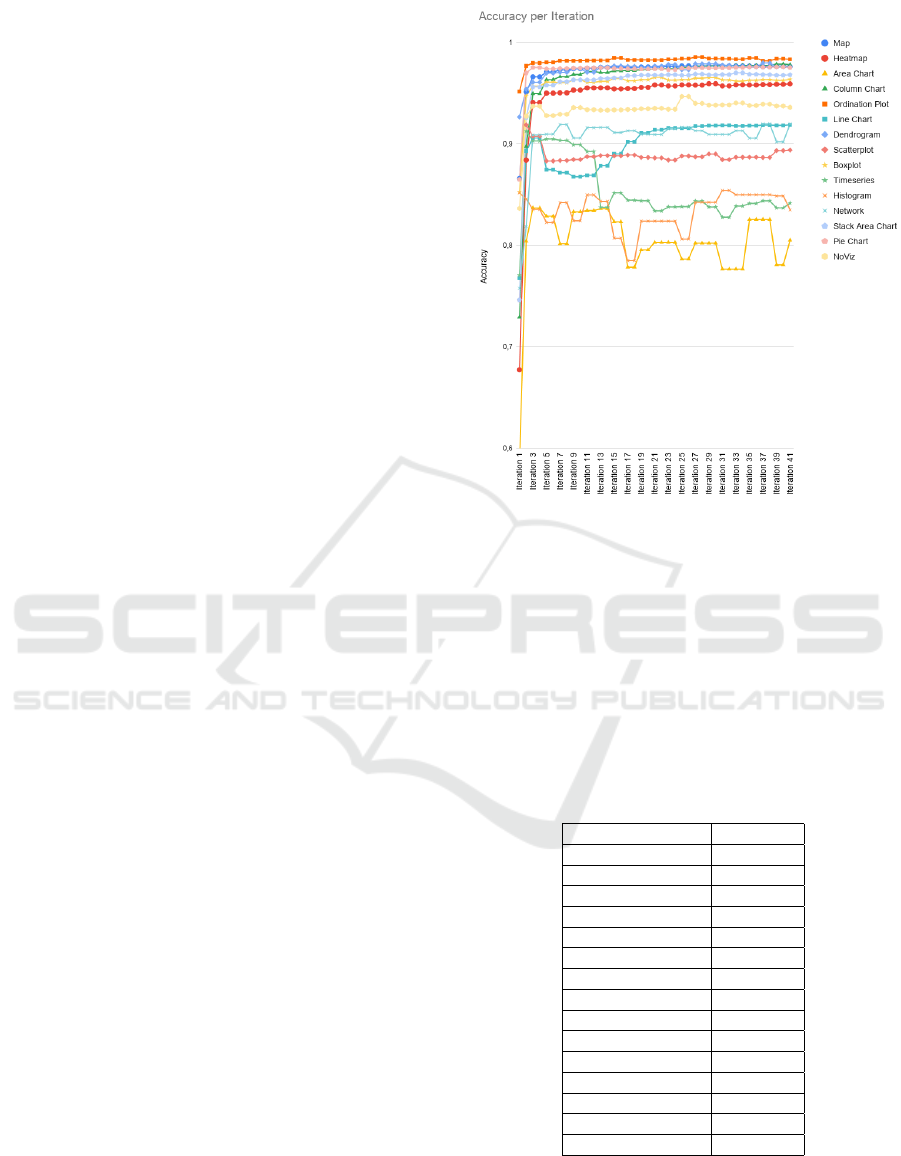
Figures 6 and 7 show the development of the quality

of the classiﬁers as well as the number of samples for

each label over the course of the 41 iterations neces-

sary to reach the ending criterion (a tag rate of less

then 0.01 % of the unlabeled samples of the corpus).

In most cases, the quality of the classiﬁers rises the

most within the ﬁrst 3 iterations. After that phase,

most classiﬁers do not change in quality any more.

Exceptions are the line chart, with a drop after the

steep rise in the beginning, the time series, with a drop

at the eleventh iteration, and the histogram and area

charts that ﬂuctuate around 80% accuracy. The drops

in the performances of both line chart and time series

classiﬁers coincide with steep rises in the numbers of

examples for the respective classes, suggesting that

the classiﬁer needed some iterations to adapt to the

new dataset. The ﬂuctuations in the quality of his-

togram and area chart classiﬁers stem from the small

sample sizes for the respective classes. For the confu-

sion matrix, please refer to Section 5 of appendix.

We have found the most consistent confusions be-

tween boxplots and column charts and maps and pie

charts. The confusion between boxplots and column

charts could stem from the presence of error bars in

boxplots and a special type of column charts. The

confusion between maps and pie charts could be ex-

plained with the presence of certain images where pie

charts were overlaid on the maps. Another similar

Figure 6: Line graph of the development of the accuracy

of each binary classiﬁer during the iterative learning phase.

Notably, even though most classiﬁers began with classiﬁca-

tion accuracy of less than 80%, almost all of them increase

their accuracy drastically after the ﬁrst ﬁve iterations.

case is between pie charts and stacked area charts.

The reason could be because both visualizations share

a similar representation goal as ’Proportion’ and the

division of some examples from ’Proportion’ into

these two charts at the previous stage (see subsubsec-

tion 4.3.4).

Table 5: Scores from Incremental Learning.

Classes Accuracy

Ordination Plot 0.98

Map 0.97

Scatterplot 0.89

Line Chart 0.91

Dendrogram 0.97

Column Chart 0.97

Heatmap 0.95

Boxplot 0.96

Area Chart 0.80

Network 0.91

Histogram 0.83

Timeseries 0.84

Noviz 0.93

Pie Chart 0.97

Stack Area Chart 0.96

Combining Image and Caption Analysis for Classifying Charts in Biodiversity Texts

165

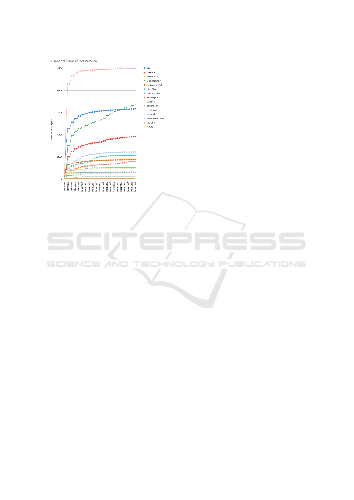
Figure 7: The development of the sample sizes for each

class during the iterative annotation. Similar to the increase

in accuracy of the binary classiﬁers in Figure 6, the numbers

of sample sizes increase very quickly within the ﬁrst few

iterations.

5.2 Reasons for Misclassiﬁcations

In our extensive study of the misclassiﬁcation cases,

we were able to extract several categories of reasons,

why these misclassiﬁcations happened.

• Mixed Vocabulary from Different Chart

Types: The main reasons for this problem was

a) often, multiple different visualizations are

used in conjunction in one image, showing, for

example, pie charts on different locations on a

map. We have observed that the classiﬁer could

not perform well on those image captions, as

the information about multiple chart types in the

same text seemed to offer conﬂicting clues. b)

In one image, multiple different visualizations

are used to represent multidimensionality of

the results. For example, the use of scatterplot

for showing the distribution of some species

and in the same image use of column chart for

illustrating the comparison with other species.

Although all efforts were made to remove such

instances from our training set, however, we

can’t deny the existence of them in the rest of the

corpus.

• Similar Representational Goal: Histograms,

boxplot and scatterplot share same goal of

showing distribution among continuous variables.

Where histogram shows the frequency distribu-

tion of a variable, boxplot provides detail informa-

tion about this distribution among different quar-

tiles. Then, scatterplot shows relationship and

causation of this distribution with other variable/s.

Unfortunately, although the visual representation

is different, the language describing both visual-

izations tends to use similar wording, likely caus-

ing misclassiﬁcations.

• Mixture of Deﬁnition/Description and Inter-

pretation Vocabulary: A caption can be used

to fulﬁll different tasks: deﬁne/describe the con-

tents and/or interpret them. As the language dif-

fers very heavily from one task to the other and

the ratio between deﬁnitions and interpretations

varies from sample to sample even within a given

class, a classiﬁer might be drawn to either spe-

cialize in the deﬁnition/interpretation parts of the

samples (high precision, low recall) or generalize

to a point that it cannot exclude other classes (low

precision, high recall).

• Level of Abstraction of Some Classes: Due

to limited examples for some of the classes, we

had to form superclasses of visualization types.

For example, ’Column Chart’ class is created

by merging examples from 14 related visual-

izations. This also leads confusion with other

classes. For example boxplots are confused with

column charts due to the presence of error bars in

certain types of column chart.

• Wrongly Mentioned Visualization Types: In

addition to the regular vocabulary, the binary clas-

siﬁers also look for speciﬁc visualization name in

the caption texts. Unfortunately, in some captions,

wrong visualization names are referred, mistaking

for example a column chart for a histogram.

5.3 Comparison

Table 5 provides individual scores for different

classes. Due to the special goal and characteristics

of our study, currently we do not have any base study

to compare our results with. None of the previous

studies have considered both aspects of charts (visu-

als from images and chart semantics from captions)

for chart classiﬁcation. In Figure 8, we have provided

the comparison among scores from common classes

in 3 different studies.

Figure 8 shows that in comparison to other stud-

ies, we are only lacking in two classes i.e Scatterplot

and Area Chart. In our work, ’Ordination Plot’ and

’Stack Area Chart’ which is similar to ’Scatterplot’

IVAPP 2020 - 11th International Conference on Information Visualization Theory and Applications

166

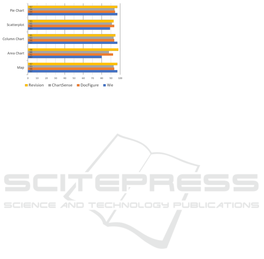
Figure 8: Comparison with other studies: Revision (Savva

et al., 2011), ChartSense (Jung et al., 2017) and DocFigure

(Jobin et al., 2019).

and ’Area Chart’ were considered as a separate class

based on their representative goal and visual dissim-

ilarities. No such ﬁne differences were made in the

other studies. Scores of Ordination plot is 98% and

Stack area chart score 96% and if we compare them

with the other studies, then our performance is bet-

ter. With an average accuracy (F1-score) of 92.2%

we have proved that our approach of chart classiﬁ-

cation is better than other chart image classiﬁcation

technique.

6 CHALLENGES AND

RESEARCH DIRECTION

The result from our study lays a strong foundation that

for better chart classiﬁcation apart from visual chart

elements, caption and other chart related text could

be a major source of information.It is just a prelim-

inary step. For an enhanced semantic chart recogni-

tion systems, there are many problems that needs to

be answered-

• As our classiﬁers were only trained on the biodi-

versity text, we are not sure how well they will

perform on general text or text from other do-

mains. More studies are needed in this direction

wherein a classiﬁer trained in one domain can be

generalized to other domain. This work is out of

scope for our research therefore, we leave it on

future studies.

• Apart from only using the captions in the train-

ing process, text in the publication refers to the

chart images could yield better results. Moreover,

if the data is enriched with more semantic knowl-

edge like synonyms, concurrent words, ontolo-

gies etc, then better classiﬁcation accuracy can be

achieved.

• The real population is not always as clean as the

training data that is fed to the classiﬁers. There-

fore, more studies are required that can under-

stand the common variations found in the visual-

ization images and captions. For example, hybrid

visualizations, multi-embed visualizations etc.

• Semantic chart classiﬁcation classify the charts

not only based on the chart elements but also their

representation goals. We have found that those vi-

sualizations that tend to share the same goals are

the one with most false positives. The way out for

this is to create the classes solely based on the vi-

sualization goals. Then such work will be more

helpful for task-based visualization recommenda-

tion systems.

7 CONCLUSION AND FUTURE

WORK

In this work on chart classiﬁcation, along with the vi-

sual similarity of different chart types, we have also

considered the conceptual similarities of the charts.

We have manually labelled the chart images and cap-

tions from biodiversity publications. We have trained

both the image and chart classiﬁers on this data. From

the best results of these two classiﬁers, we have in-

crementally trained our text classiﬁer. Doing so,

we have achieved an average (F1-score) of 92.2%

from ensembles of binary caption classiﬁers. Our re-

sult proves that conceptual/semantic chart classiﬁers

can efﬁciently differentiate between those chart types

which are visually similar and are as efﬁcient as im-

age classiﬁers. Along with that due to the conceptual

understanding of such classiﬁers, they can be used

for different purposes. One of these is the creation

of knowledge-assisted visualization recommendation

systems. We will be using these classiﬁers to infer

different visualizations/chart types from biodiversity

text.

ACKNOWLEDGEMENTS

The work has been funded by the DFG Priority Pro-

gram 1374 Infrastructure-Biodiversity-Exploratories

(KO 2209 / 12-2). We would like to thanks our

project principal investigator Birgitta K

onig-Ries for

her valuable feedback.

Combining Image and Caption Analysis for Classifying Charts in Biodiversity Texts

167

REFERENCES

(2018). Elsevier sciencedirect apis. https://dev.elsevier.

com/sciencedirect.html#/Article Retrieval.

(2019). https://tfhub.dev/google/imagenet/mobilenet v2

050 96/feature vector/2.

Abadi, M., Agarwal, A., Barham, P., Brevdo, E., Chen, Z.,

Citro, C., Corrado, G. S., Davis, A., Dean, J., Devin,

M., et al. (2016). Tensorﬂow: Large-scale machine

learning on heterogeneous distributed systems. arXiv

preprint arXiv:1603.04467.

Abhijit Balaji, Thuvaarakkesh Ramanathan, V. S. (2018).

Chart-text: A fully automated chart image descriptor.

CoRR, abs/1812.10636.

Aggarwal, C. C. and Zhai, C. (2012). Mining text data.

Springer Science & Business Media.

Boser, B. E., Guyon, I. M., and Vapnik, V. N. (1992).

A training algorithm for optimal margin classiﬁers.

In Proceedings of the 5th Annual ACM Workshop

on Computational Learning Theory, pages 144–152.

ACM Press.

Charbonnier, J., Sohmen, L., Rothman, J., Rohden, B., and

Wartena, C. (2018). Noa: A search engine for reusable

scientiﬁc images beyond the life sciences. In Pasi, G.,

Piwowarski, B., Azzopardi, L., and Hanbury, A., ed-

itors, Advances in Information Retrieval, pages 797–

800, Cham. Springer International Publishing.

Chen, M., Grinstein, G., Johnson, C. R., Kennedy, J., and

Tory, M. (2017). Pathways for theoretical advances in

visualization. IEEE computer graphics and applica-

tions, 37(4):103–112.

Chollet, F. et al. (2015). Keras. https://keras.io.

Cortes, C. and Vapnik, V. (1995). Support-vector networks.

In Machine Learning, pages 273–297.

Goodfellow, I., Bengio, Y., and Courville, A. (2016). Deep

Learning. MIT Press. http://www.deeplearningbook.

org.

Harris, R. L. (2000). Information graphics: A comprehen-

sive illustrated reference. Oxford University Press.

Ho, T. K. (1995). Random decision forests. In Proceedings

of 3rd international conference on document analysis

and recognition, volume 1, pages 278–282. IEEE.

Joachims, T. (1998). Text categorization with support vec-

tor machines: Learning with many relevant features.

In European conference on machine learning, pages

137–142. Springer.

Jobin, K. V., Mondal, A., and Jawahar, C. V. (2019).

Docﬁgure: A dataset for scientiﬁc document ﬁgure

classiﬁcation. In 2019 International Conference on

Document Analysis and Recognition Workshops (IC-

DARW), volume 1, pages 74–79.

Jung, D., Kim, W., Song, H., Hwang, J.-i., Lee, B., Kim,

B., and Seo, J. (2017). Chartsense: Interactive data

extraction from chart images. In Proceedings of the

2017 CHI Conference on Human Factors in Comput-

ing Systems, pages 6706–6717. ACM.

Kaur, P., Klan, F., and K

onig-Ries, B. (2018). Issues and

suggestions for the development of a biodiversity data

visualization support tool. In Proceedings of the Eu-

rographics/IEEE VGTC Conference on Visualization:

Short Papers, EuroVis ’18, pages 73–77.

Kingma, D. P. and Ba, J. (2014). Adam: A

method for stochastic optimization. arXiv preprint

arXiv:1412.6980.

Lee, P.-s., West, J. D., and Howe, B. (2017). Viziometrics:

Analyzing visual information in the scientiﬁc litera-

ture. IEEE Transactions on Big Data, 4(1):117–129.

Liu, Y., Lu, X., Qin, Y., Tang, Z., and Xu, J. (2013). Review

of chart recognition in document images. In Visualiza-

tion and Data Analysis 2013, volume 8654, pages 384

– 391. International Society for Optics and Photonics,

SPIE.

Moody, A. and Jones, J. A. (2000). Soil response to canopy

position and feral pig disturbance beneath quercus

agrifolia on santa cruz island, california. Applied Soil

Ecology, 14(3):269 – 281.

Munzer, T. (2009). A nested model for visualization design

and validation. IEEE Transactions on Visualization

and Computer Graphics, 15(6):921–928.

Murphy, R. F., Kou, Z., Hua, J., Joffe, M., and Cohen,

W. W. (2004). Extracting and structuring subcellu-

lar location information from on-line journal articles:

The subcellular location image ﬁnder. In Proceedings

of the IASTED International Conference on Knowl-

edge Sharing and Collaborative Engineering, pages

109–114.

Rafkind, B., Lee, M., Chang, S.-F., and Yu, H. (2006).

Exploring text and image features to classify im-

ages in bioscience literature. In Proceedings of the

HLT-NAACL BioNLP Workshop on Linking Natural

Language and Biology, LNLBioNLP ’06, pages 73–

80, Stroudsburg, PA, USA. Association for Computa-

tional Linguistics.

Ramos, J. et al. (2003). Using tf-idf to determine word rele-

vance in document queries. In Proceedings of the ﬁrst

instructional conference on machine learning, volume

242, pages 133–142. Piscataway, NJ.

Sandler, M., Howard, A., Zhu, M., Zhmoginov, A., and

Chen, L. (2018). Inverted residuals and linear bottle-

necks: Mobile networks for classiﬁcation, detection

and segmentation. arXiv preprint arXiv:1801.04381.

Savva, M., Kong, N., Chhajta, A., Fei-Fei, L., Agrawala,

M., and Heer, J. (2011). Revision: Automated clas-

siﬁcation, analysis and redesign of chart images. In

Proceedings of the 24th annual ACM symposium on

User interface software and technology, pages 393–

402. ACM.

Sebastiani, F. (2002). Machine learning in automated

text categorization. ACM computing surveys (CSUR),

34(1):1–47.

Srihari, R. K. (1991). Piction: A system that uses captions

to label human faces in newspaper photographs. In

AAAI, pages 80–85.

Xu, S., McCusker, J., and Krauthammer, M. (2008). Yale

image ﬁnder (yif): a new search engine for retriev-

ing biomedical images. Bioinformatics, 24(17):1968–

1970.

APPENDIX

Appendix and scripts are available online at:

https://github.com/fusion-jena/Biodiv-Visualization-

Classiﬁer

IVAPP 2020 - 11th International Conference on Information Visualization Theory and Applications

168