
Efficient Stereo Matching Method using Elimination of Lighting
Factors under Radiometric Variation
Yong-Jun Chang
1a
, Sojin Kim
2
, and Moongu Jeon
1,2 b
1
School of Electrical Engineering and Computer Science, Gwangju Institute of Science and Technology (GIST),
Gwangju, South Korea
2
Korea Culture Technology Institute (KCTI), Gwangju Institute of Science and Technology (GIST), Gwangju, South Korea
Keywords: Stereo Matching, Color Formation Model, Local Binary Patch, Radiometric Variation.
Abstract: Many stereo matching methods show quite accurate results from depth estimation for images captured under
the same lighting conditions. However, the lighting conditions of the stereo image are not the same in the real
video shooting environment. Therefore, stereo matching, which estimates depth information by searching
corresponding points between two images, has difficulty in obtaining accurate results in this case. Some
algorithms have been proposed to overcome this problem and have shown good performance. However, those
algorithms require a large amount of computation. For this reason, they have a disadvantage of poor matching
efficiency. In this paper, we propose an efficient stereo matching method using a color formation model that
takes into account exposure and illumination changes of captured images. Our method changes an input image
to a radiometric invariant image and also applies a local binary patch, which is robust to lighting changes, to
the transformed image according to exposure and illumination changes to improve the matching speed.
1 INTRODUCTION
Many researchers have studied techniques for
providing more realistic video content to the public.
This effort led to the development of high-resolution
digital imaging technologies such as high definition
television (HDTV) and ultra high definition
television (UHDTV). In addition, since the late
2000s, three-dimensional (3D) movies have been
popular all over the world, and various types of 3D
video content have been produced. Recently,
techniques for creating immersive video content such
as super multi-view images and 360° images are also
being studied. Various image processing and
computer vision theories are used to create such
realistic and immersive video content, and depth
information of the object plays an important role in
adding realism to the two-dimensional (2D) image.
The more accurate the depth information of the
object, the more realistic 3D video content can be
produced. Therefore, until recently, research to obtain
accurate depth information has been actively
conducted.
a
https://orcid.org/0000-0002-1650-7311
b
https://orcid.org/0000-0002-2775-7789
One of the methods for depth estimation is an
active-sensor based method. This method uses an
infrared-ray or a laser to measure the distance
between the sensor and the object. The other method
is a passive-sensor based method. This method
estimates depth information based on geometric
theory and human visual system from single or
binocular images. One representative passive-sensor
based method is stereo matching that uses the
characteristic of binocular disparity. It compares
brightness values of pixels between two images
having different viewpoints. Then, corresponding
points are found and the disparity value between them
is calculated. According to the characteristic of
binocular disparity, the disparity value is interpreted
as depth information of that pixel.
There are several ways to estimate disparity
values using stereo matching. A local stereo matching
method defines a cost function between a reference
patch and a target patch in the stereo image. After
that, the principle of winner-takes-all (WTA) is
applied to the matching cost calculated for all
disparity candidates to determine the optimal
disparity value of the current pixel. This is the basic
Chang, Y., Kim, S. and Jeon, M.
Efficient Stereo Matching Method using Elimination of Lighting Factors under Radiometric Variation.
DOI: 10.5220/0008945307750782
In Proceedings of the 15th International Joint Conference on Computer Vision, Imaging and Computer Graphics Theory and Applications (VISIGRAPP 2020) - Volume 4: VISAPP, pages
775-782
ISBN: 978-989-758-402-2; ISSN: 2184-4321
Copyright
c
2022 by SCITEPRESS – Science and Technology Publications, Lda. All rights reserved
775

method for disparity estimation from the stereo
image. Recently, a method for improving the
performance of local stereo matching by aggregating
the matching cost calculated according to the
disparity candidates has been proposed (Zhang et al.,
2014). Another type of stereo matching is a global
stereo matching method. This method models an
energy function for the disparity estimation. The
energy function includes a data term and a
smoothness term. Each of the terms calculates the
matching cost and checks the disparity continuity
among neighboring pixels, respectively. This
function is optimized by some optimization
algorithms such as belief propagation (Sun et al.,
2002) and graph cuts (Boykov et al., 2001) to
determine the final disparity value. Generally, the
global stereo matching method shows better
performance than the local stereo matching method.
However, due to the process of optimization that
compares the disparity continuity among pixels, this
method usually requires more computation than the
local stereo matching method.
Recently, many researchers are interested in deep
learning, and since the appearance of AlexNet
(Krizhevsky et al., 2012), researches on image
processing and computer vision using convolutional
neural networks (CNNs) such as VGGNet (Simonyan
et al., 2014) and ResNet (He et al., 2016) have
increased. Those networks have been applied to
various fields in computer vision and shown better
performance than conventional methods. At a similar
time, deep learning began to be used for stereo
matching. MC-CNN calculates the matching cost by
extracting the same sized patch from the left and right
viewpoint images according to disparity candidates.
Then, it trains the learning model to have the optimal
matching cost at the actual disparity value (Z
bontar et
al., 2015). Similarly, an algorithm was proposed that
improves the performance of MC-CNN by increasing
the size of the target patch according to disparity
candidates and then training the probability
distribution of the matching cost (Luo et al., 2016).
Those two methods applied deep learning only to the
part that calculates the matching cost in stereo
matching. Unlike those methods, a method of
applying deep learning to all the processes of stereo
matching was proposed (Mayer et al., 2016).
Although many stereo matching papers have been
published so far, most stereo matching algorithms
have been tested to stereo images taken under the
same lighting conditions. In a real stereo image
shooting environment, it is difficult for two viewpoint
images to have the same lighting conditions and it
causes errors in the result of stereo matching. An
adaptive normalized cross-correlation (ANCC) that
calculates the matching cost between two images by
eliminating lighting factors in the color formation
model was proposed (Heo et al., 2010). This method
shows a stereo matching result that is robust to
lighting changes. However, in calculating the
matching cost, there is a disadvantage that it is
inefficient because of too much computational
complexity. Various methods have been proposed to
solve the computational complexity problem of
ANCC. Those methods have less computational
complexity than that of ANCC. However, they show
unstable stereo matching results compared with
ANCC. Therefore, we propose an efficient stereo
matching method that shows fast and stable matching
results for various lighting changes.
2 RELATED WORKS
In general, the result of stereo matching is poor when
images are captured under different lighting
conditions. Fig. 1 shows results of stereo matching
with various methods. We tested conventional stereo
matching methods using Aloe from Middlebury
stereo datasets (Scharstein et al., 2007).
(a) Left image (b) Right image (c) SAD
(d) DL (e) NCC (f) Ground truth
Figure 1: Stereo matching with various methods.
In Fig. 1, Fig. 1(a) and (b) represent a left
viewpoint and a right viewpoint images. Both images
are captured under different illumination conditions.
Fig. (c) - (e) show stereo matching results using the
sum of absolute differences (SAD), deep learning
(Luo et al., 2016), and normalized cross-correlation
(NCC), respectively. Fig. (f) is a ground truth
disparity map of the left viewpoint image. All results
in Fig. 1 were optimized by graph cuts (Boykov et al.,
2001). As shown in Fig. 1, it is difficult to obtain a
good disparity map with general matching methods.
Even the stereo matching method using deep learning
shows a poor disparity map. In this section, we
introduce some algorithms proposed to solve this
VISAPP 2020 - 15th International Conference on Computer Vision Theory and Applications
776

problem and also explain disadvantages of each
method.
2.1 Adaptive Normalized
Cross-Correlation (ANCC)
The ANCC method (Heo et al., 2010) uses a color
formation model that is defined by (Finlayson et al.,
2003) to remove lighting factors from captured
images. The color formation model in the left
viewpoint image is defined in (1). In the process of
storing a digital image, the actual color values are
distorted by lighting factors as shown in (1).
𝑅
𝑝
𝐺
𝑝
𝐵
𝑝
→
𝑅
𝑝
𝐺
𝑝
𝐵
𝑝
𝜌
𝑝
𝑎
𝑅
𝑝
𝜌
𝑝
𝑏
𝐺
𝑝
𝜌
𝑝
𝑐
𝐵
𝑝
(1)
In (1), where 𝜌
𝑝
is a brightness factor that
represents the lighting geometry at the current pixel
𝑝, 𝛾
is a gamma exponent, and 𝑎
, 𝑏
, and 𝑐
are
scale factors. The ANCC removes 𝜌
𝑝
using log-
chromaticity normalization. As a result, 𝑅
𝑝
is
changed to (2).
𝑅
𝑝
log
𝛾
log
(2)
There are still scale factors and the gamma
exponent in (2). ANCC uses a N×N sized patch for
elimination of scale factors. It also applies a bilateral
filter to the patch (Tomasi et al., 1998) for preserving
depth information of object boundary. An equation
for removing scale factors is defined in (3).
𝑅
𝑡
𝑅
𝑡
∑
𝑤
𝑡
𝑅
𝑡
∈
𝑍
𝑝
(3)
In (3), where 𝑊
𝑝
is the kernel at current pixel
𝑝, 𝑤 represents the kernel of bilateral filter, and 𝑍
means the sum of weights in the bilateral kernel. The
last lighting factor, the gamma exponent, is removed
using an equation of NCC as shown in (4).
𝐴𝑁𝐶𝐶
_
𝑓
∑
𝑤
𝑡
𝑤
𝑡
𝑅
𝑡
×
𝑅
𝑡
∑|
𝑤
𝑡
𝑅
𝑡
|
×
∑|
𝑤
𝑡
𝑅
𝑡
|
(4)
The equation (4) is used as a cost function of
ANCC. In (4), where 𝐴𝑁𝐶𝐶
_
means the cost
function of log 𝑅 channel and 𝑓
is a set of disparity
candidates at the current pixel. This cost function
shows robust results in lighting changes. Authors of
ANCC define an additional cost function from the
original RGB image to compensate the information
loss due to the process of log-chromaticity
normalization. The cost function of original 𝑅
channel is defined in (5). In (5), where 𝑅
𝑡
𝑅
𝑡
∑
∈
.
𝐴
𝑁𝐶𝐶
𝑓
∑
×
∑|
|
×
∑|
|
(5)
Both cost functions in (4) and (5) are applied to
the energy function for the global stereo matching,
and it is optimized by graph cuts.
The ANCC method using both log-chromaticity
and original RGB cost functions shows stable results
under different lighting conditions as depicted in Fig.
2(a). However, since the bilateral filter is applied to
all the pixels, the computational complexity becomes
high depending on the kernel size.
2.2 Normalized Cross-correlation in
Log-RGB Space
To reduce the computational complexity of ANCC, a
stereo matching method in log-RGB space using
NCC was proposed (Li, 2012). Unlike ANCC, which
requires the bilateral filter for all pixels in the image
to remove scale factors, this method has less
computational complexity than ANCC because it
only requires calculating the average of all the pixel
values in the log-RGB image. Therefore, the equation
of (3) is changed to (6). In (6), where 𝐼
is a set of
pixels in the log-RGB image having the left
viewpoint and 𝑀 is the number of pixels in the image.
𝑅
𝑡
𝑅
𝑡
∑
𝑅
𝑡
∈
𝑀
(6)
(a) ANCC (b) Log-RGB (c) APBM
Figure 2: Results of ANCC, Log-RGB, APBM methods.
The removal of the remaining lighting factor is the
same as that of ANCC. We implemented this method
and tested it using the same image used in Fig. 1. The
result of this method is shown in Fig. 2(b). Compared
with the ANCC result in Fig. 2(a), the result of this
method looks worse. On the contrary, compared with
Efficient Stereo Matching Method using Elimination of Lighting Factors under Radiometric Variation
777

the results of Fig. 1(c), (d), and (e), Fig. 2(b) shows a
better result than them.
2.3 Adaptive Pixel-wise and
Block-wise Matching (APBM)
An adaptive pixel-wise and block-wise matching
(APBM) is another stereo matching method that has
lower computational complexity than ANCC and is
robust to lighting changes (Chang et al., 2019). This
method removes scale factors using the average of the
all the pixel values in the log-RGB image and
eliminates the gamma exponent using an equation of
hue transformation. Through this process, the input
image is converted into an independent image from
the lighting factors.
The APBM method uses the equation of pixel-
wise matching based on the transformed input image
to speed up the process of stereo matching.
Subsequently, the equation of block-wise matching is
also used for compensation of the matching
inaccuracy caused by using the pixel-wise matching.
This method is faster than ANCC. However, when we
compare the APBM result with the result obtained
using both log-chromaticity and original RGB cost
functions, the result of APBM looks worse than that
of ANCC as depicted in Fig. 2(c).
3 PROPOSED METHOD
3.1 Analysis of Conventional Methods
In Section 2, we introduced ANCC that showed
robust stereo matching results in various lighting
conditions and also introduced Log-RGB and APBM
methods that solve the computational complexity
problem of ANCC. However, those algorithms did
not show better results than ANCC in terms of stereo
matching accuracy. For the objective evaluation of
each algorithm, we estimated disparity maps by
applying each algorithm to Aloe images captured
under various exposure and illumination. After that,
the error rate between the obtained disparity map and
the ground truth was calculated and summarized in
Table 1 and Table 2.
Table 1 shows an error rate comparison under
different exposure levels and Table 2 represents the
error rate comparison under different illumination
levels. Each first column in the two tables means the
exposure and the illumination levels of the left and
right images, respectively. In Table 1, where GC
means that the energy function is optimized by graph
cuts. ANCC, Log-RGB, and APBM methods show
lower error rates than SAD when the two images have
different exposure levels. However, when compared
to NCC, those methods show higher error rates than
NCC. In particular, at dark exposure levels (e.g. 0-0,
0-1, and 0-2), those methods show very poor results
than NCC.
On the other hand, it can be seen that ANCC, Log-
RGB, and APBM methods show better error rates for
most illumination levels than SAD and NCC.
Especially, those methods perform better than other
methods when the illumination level differences
between the left and right images are large (e.g. 1-3
and 2-3).
Table 1: Error rate comparison (exposure).
SAD
+GC
NCC
+GC
ANCC
(7×7)
ANCC
(31×31)
Log-
RGB+GC
APBM
+GC
Error rates (%)
0-0 13.9 13.05 12.27 10.74 18.32 15.3
0-1 97.87 10.96 16.24 13.6 17.94 15.32
0-2 97.93 10.75 19.55 15.48 16.73 14.33
1-1 12.01 10.23 6.6 5.42 12.46 9.19
1-2 97.55 10.13 6.22 4.99 11.19 7.62
2-2 11.09 9.94 5.37 4.5 9.99 5.51
Table 2: Error rate comparison (illumination).
SAD
+GC
NCC
+GC
ANCC
(7×7)
ANCC
(31×31)
Log-
RGB+GC
APBM
+GC
Error rates (%)
1-1 12.01 10.26 6.6 5.29 12.43 9.42
1-2 77.43 12.75 9.78 7.97 15.65 11.68
1-3 82.99 23.01 16.35 11.81 17.44 13.8
2-2 11.97 10.72 5.98 4.55 10.9 7.2
2-3 72.25 17.93 12.91 9.73 16.28 13.02
3-3 11.9 11.42 7.24 5.2 11.9 8.59
Both Table 1 and Table 2 show that ANCC, Log-
RGB, and APBM are generally stronger than SAD
and NCC for illumination changes, but are more
vulnerable to exposure changes. In the case of the
NCC method, it shows robust results in exposure
changes without removing lighting factors of input
images. Therefore, ANCC, Log-RGB, and APBM
methods, which remove lighting factors from input
images based on the color formation model, are rather
inefficient compared to NCC.
The purpose of proposed method is to create an
efficient stereo matching algorithm that uses basic
and simple cost functions to reduce computational
complexity and is also robust to exposure and
illumination changes.
VISAPP 2020 - 15th International Conference on Computer Vision Theory and Applications
778
3.2 Image Transformation
We analyzed that APBM performed worse than
ANCC because it did not consider the problem of
discriminability caused by the log-chromaticity
normalization, which was mentioned in the original
paper of ANCC. Therefore, the proposed method
transforms the input image to the independent image
from lighting factors based on color formation models
divided into two cases to solve this problem.
The first case is that the stereo image is captured
with a fixed camera exposure. In this case, we assume
that scale factors in (1) are all the same. According to
this assumption, (1) is rewritten as (7).
𝑅
𝑝
𝐺
𝑝
𝐵
𝑝
→
𝑅
𝑝
𝐺
𝑝
𝐵
𝑝
𝜌
𝑝
𝑅
𝑝
𝜌
𝑝
𝐺
𝑝
𝜌
𝑝
𝐵
𝑝
(7)
In the same way with ANCC, the log transform is
applied to (7). After that, the log-chromaticity
normalization is performed for eliminating the
brightness factor. Therefore, an equation (2) is
changed to (8).
𝑅
𝑝
𝛾
log
𝑅
𝑝
𝑅
𝑝
𝐺
𝑝
𝐵
𝑝
(8)
The second case is that the stereo image is
captured with a fixed lighting geometry. In this case,
the brightness factor 𝜌
𝑝
may be omitted from (1).
Therefore, we assume that the color formation model
in (1) is transformed to (9).
𝑅
𝑝
𝐺
𝑝
𝐵
𝑝
→
𝑅
𝑝
𝐺
𝑝
𝐵
𝑝
𝑎
𝑅
𝑝
𝑏
𝐺
𝑝
𝑐
𝐵
𝑝
(9)
In (9), there are scale factors 𝑎
, 𝑏
, and 𝑐
. We
apply log transform to (9). The scale factors are
removed by subtracting the average pixel value of
each color channel from all the pixels in the log image.
Those processes are defined in (10) and (11). The
equation (11) is also summarized in (12).
log
𝑅
𝑝
log𝑎
𝛾
log𝑅
𝑝
(10
)
𝑅
𝑝
log
𝑅
𝑝
∑
∈
(11)
𝑅
𝑝
𝛾
log
∏
∈
(12)
The proposed method uses the average sum of (8)
and (11) to solve the problem of discriminability. This
is because the equation (8) has the log-chromaticity
normalization problem, but (12) is free from this. The
combination of (8) and (11) is defined in (13).
In (13), there is a gamma exponent. To remove the
gamma exponent, we apply the log transformation
again to (13). After that, the gamma exponent is
removed in the same manner as in (11). This is
defined in (14). If the result value of (13) has a
negative value, the log transformation in (14) cannot
have real value. Therefore, in the actual
implementation process, we add the positive constant
value to (13) and apply this value to (14).
𝑅
𝑝
0.5∗𝛾
log
∙
∏
∈
(13)
𝑅
𝑝
log𝑅
𝑝
∑
log𝑅
𝑡
∈
𝑀
(14)
Based on color values converted so far, the final
transformed color channels are shown in (15). We
change the result of (14) to an exponential value. This
is because the result of (14) may have a negative
number because of the logarithmic value. In the actual
implementation process, we also multiply the positive
constant value to (15) for making 16bit integer value.
In (15), where 𝑅
, 𝐺
, and 𝐵
represent transformed
color channels using the proposed method.
𝑅
𝑝
𝐺
𝑝
𝐵
𝑝
𝑒
𝑒
𝑒
(15
)
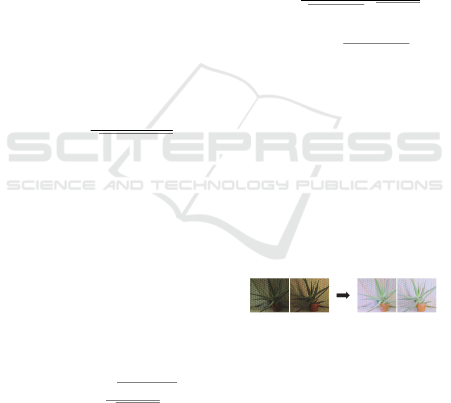
We applied our new color model to the stereo
image that was used in Fig. 1 to test. As a result,
images in Fig. 1 was changed to new images that have
similar color distributions as depicted in Fig. 3.
Figure 3: Image transformation using proposed method.
3.3 Cost Computation
The proposed method calculates the matching cost
using the transformed images in Fig. 3. For the cost
computation, we apply a census transform that uses a
local binary patch for the similarity measure between
left and right images (Zabih et al., 1994). The census
transform calculates color differences between the
center pixel and its neighboring pixels in the patch.
Subsequently, if the difference is larger than 0, the
Efficient Stereo Matching Method using Elimination of Lighting Factors under Radiometric Variation
779
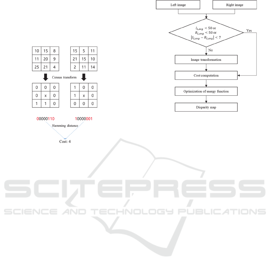
neighboring pixel value is changed to 1. In the
opposite case, that pixel value is set to 0. This process
is applied to both left and right patches. Binary values
from two patches are listed in numeric sequences as
shown in Fig. 4 to calculate the matching cost by
measuring Hamming distance.
Figure 4: Example of census transform.
The cost function calculating Hamming distance
between two patches is used as a data term 𝐷
𝑓
of
the energy function defined in (16).
𝐸
𝑓
∑
𝐷
𝑓
∑∑
𝑉
𝑓
,
𝑓
∈
(16
)
In (16), where 𝑞 is a set of neighboring pixels in
the patch and 𝑉
is a smoothness term that checks the
disparity continuity among pixels. The energy
function is optimized by graph cuts and all parameters
used in this process are the same as those used in (Heo
et al., 2010).
Table 1 shows that robust stereo matching
methods in various lighting conditions have worse
error rates than those of NCC when the exposure level
of input image is low. In addition, some algorithms in
Table 1 show worse results than NCC even under the
same exposure levels. It means that stereo matching
using the original input image shows better results
than stereo matching using the transformed image in
those situations. To solve this problem, we use
average pixel values of the left and right images and
also calculate the absolute difference between two
average values. If the average value of the left or the
right image is lower than 50, or the absolute
difference between the two average values is lower
than 7, original color images are used as inputs for
stereo matching. If not, transformed images are used.
An overall scheme of our method is shown in Fig. 5.
Figure 5: Flowchart of proposed method.
4 EXPERIMENTAL RESULTS
We tested the proposed method using Middlebury
stereo datasets: Aloe, Dolls, and Moebius (Scharstein
et al., 2007). To evaluate whether the stereo matching
result is robust to lighting changes, the exposure and
illumination levels of the left and right images were
classified into 6 cases, respectively. Fig. 6 shows
disparity maps acquired through stereo matching
methods when the illumination level of the left and
right images is 1 and 3, respectively. ‘GT’ in Fig. 6(i)
means the ground truth.
For quantitative evaluation, we measured the error
rate of the stereo matching result according to the
exposure and illumination conditions. The error rate
means that the ratio of the number of error pixels to
the total number of pixels in the image. The error
pixel refers to a pixel having the difference between
the actual disparity value and the experimentally
obtained disparity value is greater than 1. Those are
summarized in Table 3 and Table 4.
The ANCC results in Fig. 6, Table 3, and Table 4
are estimated using a 7×7 sized patch. The original
ANCC paper used a 31×31 sized patch for stereo
matching. Therefore its matching speed is slower but
results performs better than ANCC with the 7 ×7
sized patch. However, in this paper, the 7×7 sized
patch was used for the proposed method and other
methods such as SAD and NCC. For this reason, the
7 ×7 sized patch was used for ANCC for fair
comparison of execution time and error rates.
VISAPP 2020 - 15th International Conference on Computer Vision Theory and Applications
780
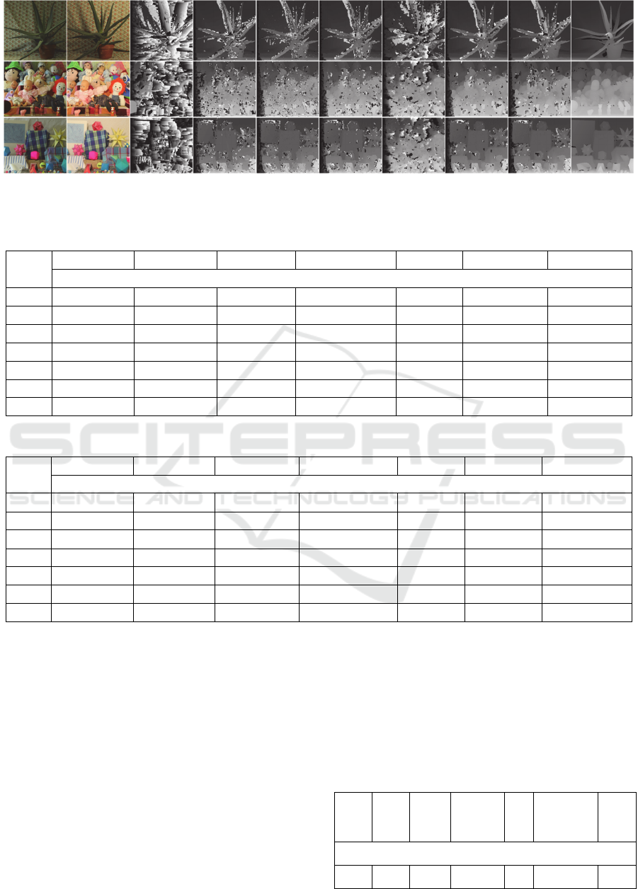
(a) Left (b) Right (c) SAD (d) NCC (e) ANCC (f) Log-RGB (g) DL (g) APBM (h) Ours (i) GT
Figure 6: Disparity maps of datasets having the illumination level of the left and right image 1 and 3, respectively.
Table 3: Error rate comparison between the proposed method and other methods (exposure).
SAD+GC NCC+GC
ANCC (7×7)
Log-RGB+GC DL APBM+GC Ours
Error rates (%)
0-0 20.33 14.55 16.48 26.06 24.25 23.88 10.03
0-1 97.93 12.71 17.82 23.51 31.11 21.07 9.17
0-2 97.99 14.6 22.3 24.64 47.17 21.96 10.63
1-1 18.14 11.56 9.46 15.86 23.56 12.31 7.04
1-2 97.47 13.22 10.34 16.63 34.79 12.25 9.13
2-2 17.23 11.66 8.03 13.2 24.94 8.63 7.19
Avg. 58.18 13.05 14.07 19.98 30.97 16.68 8.87
Table 4: Error rate comparison between the proposed method and other methods (illumination).
SAD+GC NCC+GC
ANCC (7×7)
Log-RGB+GC DL APBM+GC Ours
Error rates (%)
1-1 18.15 11.6 9.41 15.81 23.56 12.41 7.06
1-2 77.63 13.77 11.23 17.89 35.32 14.16 9.57
1-3 87.88 28.1 21.14 23.31 59.59 18.92 20.12
2-2 18.66 11.61 8.62 14.51 24.41 10.64 6.93
2-3 80.07 22.68 16.54 20.12 52.06 15.96 14.88
3-3 18.69 11.63 8.5 14.29 25.23 10.43 6.75
Avg. 50.18 16.57 12.57 17.66 36.7 13.75 10.89
Error rates in both Table 3 and Table 4 mean that
in the non-occluded region. In Table 3, where DL
means stereo matching using CNNs (Luo et al.,
2016). The proposed method shows the best results
for all exposure conditions compared to other
methods. In the case of illumination, our method
performs better in all other illumination conditions
except for ‘1-3’ than other methods as shown in Table
4.
The running time for the cost computation is
summarized in Table 5. In Table 5, the deep learning
based method shows the fastest running time.
However, as shown in Table 3 and Table 4, deep
learning-based method shows poor results for various
exposure and illumination levels. On the contrary, the
proposed method performs more robust results under
various lighting conditions than other methods. In
addition, our method shows faster cost computation
time than ANCC. Considering the error rate and the
speed of cost computation, the proposed method
shows more efficient performance than ANCC and
other methods even with the small sized patch.
Table 5: Cost computation time.
SAD
+GC
NCC
+GC
ANCC
(7×7)
Log-
RGB+GC
DL APBM+GC Ours
Time (sec.)
24.14 38.45 117.86 38.72 7.72 74.81 39.77
Efficient Stereo Matching Method using Elimination of Lighting Factors under Radiometric Variation
781

5 CONCLUSIONS
In this paper, we proposed a method for efficient
stereo matching that is robust to lighting changes and
has a fast matching speed. The proposed method
transforms the input image into the independent
image from lighting factors. After that, the matching
cost is calculated using the concept of census
transform. Besides, we also calculate average pixel
values from the left and right images. Those values
are applied to selecting whether to use the original
color image or the transformed image as an input for
stereo matching before the cost computation. As a
result, the proposed method showed three times faster
speed for the cost computation than that of ANCC and
also showed 5.2% and 1.68% lower errors than
ANCC in exposure and illumination conditions,
respectively.
ACKNOWLEDGEMENTS
This work was partly supported by Institute of Infor
mation & Communications Technology Planning &
Evaluation(IITP) grant funded by the Korea governm
ent(MSIT) (No.2014-3-00077, AI National Strategy
Project) and the National Research Foundation of Ko
rea (NRF) grant funded by the Korea government(M
SIT) (No. 2019R1A2C2087489).
REFERENCES
Zhang, K., Fang, Y., Min, D., Sun, L., Yang, S., Yan, S., &
Tian, Q. (2014). Cross-scale cost aggregation for stereo
matching. In Proceedings of the IEEE Conference on
Computer Vision and Pattern Recognition (pp. 1590-
1597).
Sun, J., Shum, H. Y., & Zheng, N. N. (2002, May). Stereo
matching using belief propagation. In European
Conference on Computer Vision (pp. 510-524).
Boykov, Y., Veksler, O., & Zabih, R. (2001). Fast
approximate energy minimization via graph cuts. IEEE
Transactions on Pattern Analysis and Machine
Intelligence, 23(11), 1222-1239.
Krizhevsky, A., Sutskever, I., & Hinton, G. E. (2012).
Imagenet classification with deep convolutional neural
networks. In Advances in Neural Information
Processing Systems (pp. 1097-1105).
Simonyan, K., & Zisserman, A. (2014). Very deep
convolutional networks for large-scale image
recognition. arXiv preprint arXiv:1409.1556.
He, K., Zhang, X., Ren, S., & Sun, J. (2016). Deep residual
learning for image recognition. In Proceedings of the
IEEE Conference on Computer Vision and Pattern
Recognition (pp. 770-778).
Zbontar, J., & LeCun, Y. (2015). Computing the stereo
matching cost with a convolutional neural network. In
Proceedings of the IEEE Conference on Computer
Vision and Pattern Recognition (pp. 1592-1599).
Luo, W., Schwing, A. G., & Urtasun, R. (2016). Efficient
deep learning for stereo matching. In Proceedings of the
IEEE Conference on Computer Vision and Pattern
Recognition (pp. 5695-5703).
Mayer, N., Ilg, E., Hausser, P., Fischer, P., Cremers, D.,
Dosovitskiy, A., & Brox, T. (2016). A large dataset to
train convolutional networks for disparity, optical flow,
and scene flow estimation. In Proceedings of the IEEE
Conference on Computer Vision and Pattern
Recognition (pp. 4040-4048).
Heo, Y. S., Lee, K. M., & Lee, S. U. (2010). Robust stereo
matching using adaptive normalized cross-correlation.
IEEE Transactions on Pattern Analysis and Machine
Intelligence, 33(4), 807-822.
Scharstein, D., & Pal., C. (2007). Learning conditional
random fields for stereo. In Proceedings of the IEEE
Conference on Computer Vision and Pattern
Recognition (pp. 1-8).
Finlayson, G., & Xu, R. (2003). Illuminant and gamma
comprehensive normalisation in logrgb space. Pattern
Recognition Letters, 24(11), 1679-1690.
Tomasi, C., & Manduchi, R. (1998). Bilateral filtering for
gray and color images. In Proceedings of the IEEE
Conference on Computer Vision (pp. 1-8)
Li, G. (2012). Stereo matching using normalized cross-
correlation in LogRGB space. In IEEE Conference on
Computer Vision in Remote Sensing (pp. 19-23).
Chang, Y. J., & Ho, Y. S. (2019). Adaptive Pixel-wise and
Block-wise Stereo Matching in Lighting Condition
Changes. Journal of Signal Processing Systems, 91(11-
12), 1305-1313.
Zabih, R., & Woodfill, J. (1994). Non-parametric local
transforms for computing visual correspondence. In
European Conference on Computer Vision (pp. 151-
158).
VISAPP 2020 - 15th International Conference on Computer Vision Theory and Applications
782
